
16 Local factor tests and the remaining bridge
On this page · Visual guide: Three mathematical objects · Visual guide: Numerical matching does not construct realization · Visual guide: Conjecture 66 isolates the missing existence claim · Visual guide: H5 compares this same actual candidate · Permalink · Source line 1814
Local class field theory identifies one dimensional Weil characters with characters of \(K^{\times}\) [27], [29]. The tame induction theorem extends this explicit picture to higher dimensional tame atoms. The local polynomial and conductor calculations in Proposition 5.4 and Proposition 5.8 therefore give explicit finite invariants for the declared tame packets. Finite Gauss sums give the residue field phase. The full local factor, however, also includes ramification depth, Haar measure normalization, the additive character conductor, and wild interaction data.
Proposition 16.1: Finite tame comparison package
For a tame induced atom, the following data are determined by its packet coordinates:
the dimension and inertia orbit
the Frobenius cycle polynomial
the Artin conductor
the local polynomial
the tensor refinement into interaction packets
the finite Gauss sum of each declared residue character, with unit-modulus phase normalization when that character is nontrivial.
Read proof · Read statement and proof side by side · Permalink · Source line 1819 · Claim record · Lean coverage · Code · Worked examples
Proof of Proposition 16.1
The dimension and orbit follow from Theorem 3.2. The cycle polynomial is Proposition 4.4. For rank greater than one, the conductor is Proposition 5.8. In rank one, the Swan conductor is zero, and the Artin conductor is zero for trivial inertia and one otherwise, by the formula \(\operatorname{Art}=\dim V-\dim V^{I_K}+\operatorname{Sw}\). The local polynomial is Proposition 5.4. Tensor refinement is Theorem 5.1. The Gauss sum is its defining finite sum; for a nontrivial multiplicative character its unit phase is Definition 6.2. For the trivial character and a nontrivial additive character \(\psi\), the sum is \(G(1,\psi)=-1\), because the sum of \(\psi\) over the whole field is zero.
Back to statement · Read statement and proof side by side · Permalink · Source line 1832 · Claim record · Lean coverage · Code · Worked examples
16.1 Arithmetic realization and the conditional comparison
On this page · Permalink · Source line 1836
Fix the paper's reciprocity, additive-character, local-factor, and phase normalizations. Let \(\mathcal A\) be the declared class of irreducible wild Weil atoms under consideration. For \(\rho\in\mathcal A\), the supplied assembled finite datum \(d_\rho\) consists of the following inputs, historically denoted H1–H4:
an intrinsic finite break decomposition on the Galois side;
the declared equivariant symplectic bridges to the supplied breakwise type-side quotients;
compatible odd or dyadic central-extension and phase data on every break, including every prescribed finite marking;
a compatible transport system with vanishing matrix holonomy obstruction.
These are finite comparison inputs. Supplying separate breakwise target types does not itself supply one common arithmetic candidate. If a common candidate is already supplied, that is a stronger restricted hypothesis.
An arithmetic realization witness \(\mathcal R(d_\rho,\pi)\) consists of actual arithmetic inducing data for an admissible supercuspidal \(\pi\), together with explicit comparison and recovery maps carrying the prescribed assembled finite packet. The maps preserve its declared stabilizer action, all character values explicitly included in the supplied datum, central-extension and phase data, and compatible transports. Recovery returns that same \(\pi\), with its fixed central character and noncompact completion. An enlarged actual inducing carrier is permitted; the whole packet is not required to be the original maximal-simple-type quotient. Any stronger native-marking or numerical-layer requirement is part of the declared datum and must be verified separately.
Conjecture 66: Arithmetic packet realization
For every \(\rho\in\mathcal A\) with its supplied H1–H4 assembled finite datum \(d_\rho\), there exists an actual admissible supercuspidal representation \(\pi\) of \({\operatorname{GL}}_{\dim\rho}(K)\) and an arithmetic realization witness \(\mathcal R(d_\rho,\pi)\).
Permalink · Source line 1871 · Claim record · Lean coverage · Code · Worked examples
This is the realization problem isolated from historical Theorem 16.2 and original proof obligation 66 (row 95 of the historical all-records register). It asks for one witness for each admitted source, rather than for success of every proposed host or every noncompact completion. No proof of the unrestricted statement is claimed.
Proposition 16.3: Comparison of one realized candidate
Let \(\rho\in\mathcal A\), and let \(\pi\) be one actual admissible supercuspidal representation of \({\operatorname{GL}}_{\dim\rho}(K)\) with \(\mathcal R(d_\rho,\pi)\). Suppose H5 holds for this same \(\pi\): its required pair local factors equal those prescribed for \(\rho\) on the stipulated characterizing family of twists, with the fixed normalizations. Assume the stated local-factor characterization applies to that family and class. Then \(\pi\) is isomorphic to the representation assigned to \(\rho\) by the established local Langlands correspondence.
Read proof · Read statement and proof side by side · Permalink · Source line 1886 · Claim record · Lean coverage · Code · Worked examples
Proof of Proposition 16.3
H5 identifies the tested local factors for this actual candidate. The applicable local-factor characterization identifies its isomorphism class with the established correspondence [18]. The realization witness ensures that it is this same candidate which carries the prescribed assembled packet. No existence conclusion is inferred from the finite gluing conditions alone.
Back to statement · Read statement and proof side by side · Permalink · Source line 1898 · Claim record · Lean coverage · Code · Worked examples
Remark 16.4
H5 remains a conditional premise about the same fixed candidate. It is not a formal consequence of the finite symplectic bridge, conductor profiles, or a choice of noncompact root. This proposition adds no unconditional pair-factor obligation to the construction conjecture.
16.2 Exact open boundary
On this page · Permalink · Source line 1914
The following issues delimit the unrestricted program. The first four construct and normalize the finite inputs for broader source classes. Conjecture 66 asks for arithmetic realization once H1–H4 are supplied. The fifth is the independent route to replacing the retained conditional H5 input.
Construct a choice free finite symplectic envelope from an arbitrary irreducible wild inertia atom, with its ramification filtration and tame stabilizer action.
Prove a canonical equivariant symplectic isometry from that envelope to the type side quotient \(J_\theta^1/H_\theta^1\).
Recover the canonical beta extension phase in every break, including the required dyadic quadratic refinement.
Prove matrix holonomy compatibility for the resulting packet transport system.
Compare the full family of pair \(L\), epsilon, and gamma factors without invoking the established correspondence.
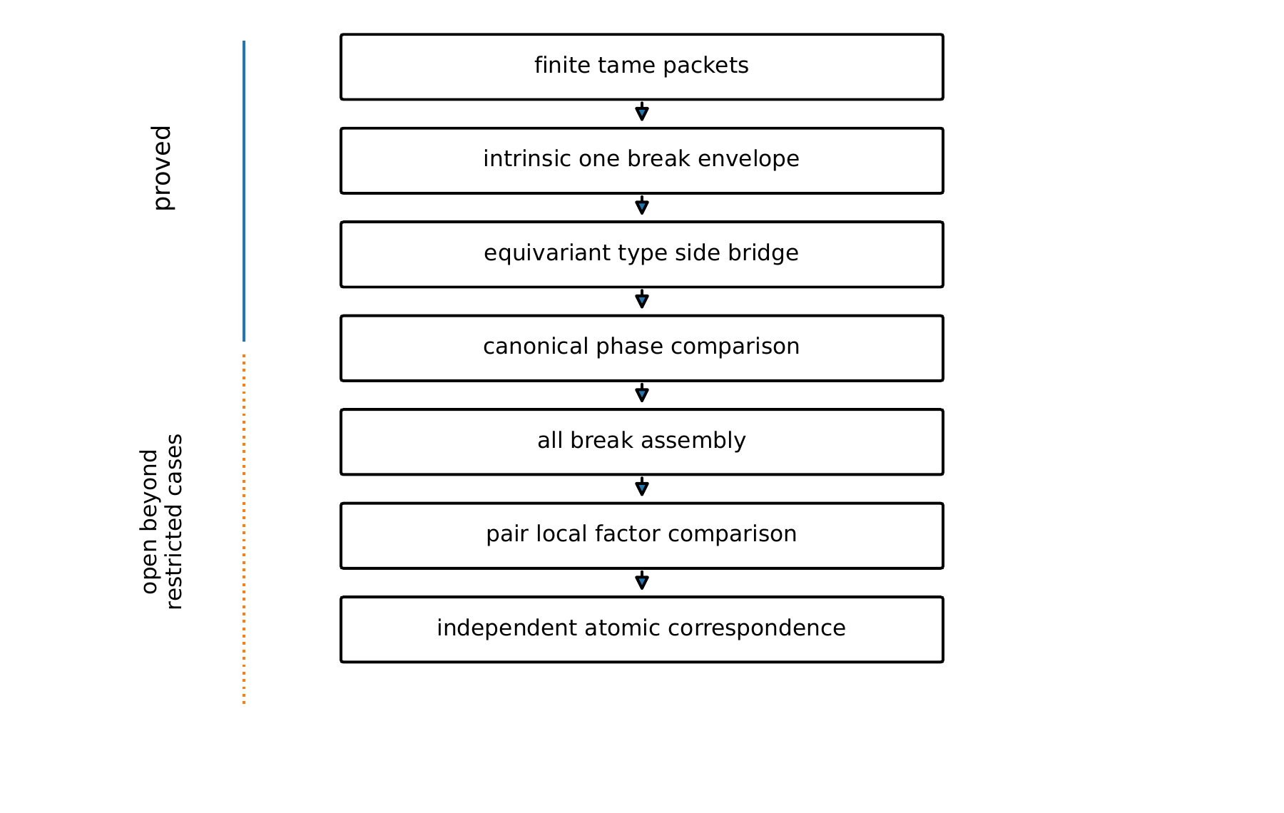
The first item is a construction problem. The second is a comparison problem. The third is a normalization problem. The fourth is a descent problem. The fifth concerns proving the local factor premise needed for identification. Conjecture 66 does not assert this fifth step. None is replaced by a larger finite computation.