A closed signal loop

The constructions become easier to distinguish when a complete example is carried through from its view equations to its obstruction, its ambiguity, and its numerical repair. The following calculations instantiate the preceding principles. They do not introduce a second, silently enlarged formal theory.

Permalink · Source line 1

Consider four scalar views arranged around a cycle. Their values are \(x_0,x_1,x_2,x_3\), and the prescribed differences are \(r_0,r_1,r_2,r_3\). Indices are taken modulo four. The compatibility equations are

Work over \({\mathbb Q}\) or \({\mathbb R}\). These equations can be presented as a strict set-valued view system: an oriented edge has pullback \(z\mapsto z-r_i\), and a path has the composite affine pullback. Use the category of paths, retaining the full loop as a path rather than imposing that it is an identity arrow in advance.

Every edge map is bijective. Around the cycle their composite is translation by \(-\sum_i r_i\). A global realization must be fixed by that translation. Thus the example makes local invertibility and global compatibility visibly different without needing a noncommutative group.

Permalink · Source line 4

Summing (33.1) gives the necessary condition

It is sufficient as well. Given an anchor \(a\), set

The first three equations hold by construction, and the last is exactly (33.2). Every solution has this form because the first three equations recursively determine it from \(x_0\). Therefore a compatible residual has a one-dimensional family of primitives, with constant shifts as its ambiguity. Prescribing the anchor removes that ambiguity.

In matrix form, the difference operator is

The explicit construction proves

Thus \(\ell\) is a complete feasibility test for this prescribed-difference problem. It annihilates every actual difference family, but takes a nonzero value on an incompatible one. This is the finite obstruction-certificate pattern of Proposition 4.2 and Proposition 35.3 in a fully visible model.

The same proof works on a cycle of any positive length: partial sums give a primitive, and the final wraparound equation is the zero-sum condition. No Fourier transform or numerical approximation is needed for this solvability argument.

Permalink · Source line 13

Take

Each of the first three edge equations can be satisfied, but the full sum is one. There is no coherent closed-loop signal with exactly these four differences. Computing a long list of partial values does not remove the missing wraparound equation.

To repair the residual, now regard the vector of edge data as a candidate in its own right. Its defect is \(\ell(r)\). The exact subspace is the zero-sum hyperplane. With the ordinary Euclidean norm and no protected edge coordinates, the nearest compatible residual is

The correction is perpendicular to the hyperplane, so the projection theorem proves it is the unique nearest vector there. Its squared size is \(1/4\). This is a repair of the edge data, not a solution of the original incompatible equations with those data unchanged.

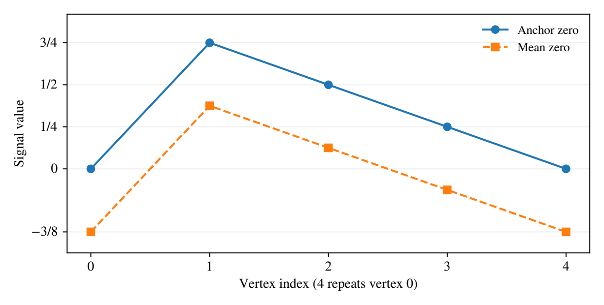
Anchor the repaired signal at zero. Its primitive is

The next partial sum is zero, so it closes. If instead the desired representative has mean zero, subtract the mean \(3/8\):

Both primitives realize exactly \(\widehat r\). They differ by an element of \(\ker D\). The anchor condition and the mean condition are two different selections from the same affine solution fiber.

Permalink · Source line 43

Suppose the first three values \((r_0,r_1,r_2)=(1,0,0)\) are required to remain fixed. The admissible corrections then affect only the final edge. Compatibility forces

for anchor zero. This is the unique repair preserving those three edges. Its squared correction size is one rather than \(1/4\). The larger error is not a failure of nearest repair: the feasible set has changed.

Here the general protected construction is completely explicit. With candidate space \(E={\mathbb R}^4\), defect \(d=\ell\), and protected observable \(p(r)=(r_0,r_1,r_2)\), the allowed direction is the last coordinate axis. The restricted operator \(d|_{\ker p}\) has gain one. Without protection, the least gain for distance to \(\ker\ell\) is \(1/2\), since \({\left\lVert\ell\right\rVert}=2\). The different constants measure different correction spaces.

Permalink · Source line 70

The raw edge family contains information about four transitions. Its zero-sum constraint links all four. Summing a block of differences transfers information to a coarser transition, while retaining the differences within the block preserves the detail that the sum omits. For example,

contains the two-step transition but does not determine \(r_0\) and \(r_1\) separately. Replacing \((r_0,r_1)\) by \((r_0+t,r_1-t)\) leaves that coarse transition unchanged.

A packet of coarse value and independent detail retains both directions. A residual-only summary can detect failure of the wraparound equation but cannot tell which protected edge may be changed. An anchor or a mean fixes the remaining signal ambiguity after feasible edge data have been chosen. These are three different roles: transition compression, feasibility repair, and representative selection.

This example is a complete finite calculation built from the strict realization, additive obstruction, and protected Hilbert principles. The companion program checks the displayed rational values, the zero-sum criterion, the primitive reconstruction, and the orthogonality equations. The calculation does not claim formal verification of a Fourier or signal-processing library.

Permalink · Source line 80

The previous cycle has scalar translations and a scalar total obstruction. A linear connection can behave differently: its loop may be nontrivial while retaining a whole subspace of feasible anchors. The following three-vertex model distinguishes full anchor preservation, feasible-anchor preservation, and global nearest-point repair in one calculation.

Permalink · Source line 91

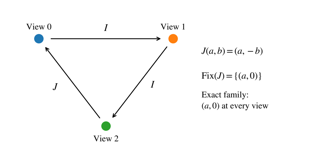
Let the fiber at each of three vertices be \({\mathbb R}^2\). Use identity transport along the route \(0\to1\to2\), and let the closing edge carry the reflection

For one chosen orientation of each edge, the residuals are

The reverse transports are inverses, so this defines an inverse-consistent isometric connection. Exactness first forces \(x_1=x_0\) and \(x_2=x_0\), and the remaining edge then forces \(Jx_0=x_0\). Hence every exact family is

The loop is not the identity on the whole fiber. Its fixed space is the first coordinate axis. Every anchor on that axis extends uniquely, and every anchor with nonzero second coordinate is obstructed if its full value is to be preserved.

The three-edge residual also gives a direct telescope:

Its second component is \(-2(x_0)_2\). In this chosen route normalization, the loop residual determines the transverse anchor component. It does not constrain the first component, which is the exact freedom seen in (34.1).

Permalink · Source line 94

Take

The measured oriented residuals are

Preserving the entire original anchor is impossible, because \((2,1)\) is not fixed by \(J\). The earlier obstruction criterion therefore gives a negative answer to that particular preservation problem.

Preserving only the feasible projection of the anchor gives a different answer. Orthogonally project \((2,1)\) to \((2,0)\), then reconstruct along the tree. The result is

It is the unique exact family preserving the first component of the original anchor. It does not preserve its second component, and makes no claim to do so.

For global nearest-point repair, declare the Euclidean product norm on \(({\mathbb R}^2)^3\). The closest member of (34.1) uses the mean of the three first coordinates, namely three:

To verify this without appealing only to a general theorem, write the squared error at parameter \(a\):

It is minimized uniquely at \(a=3\). The anchor-based answer has squared error eleven. The globally nearest answer has squared error eight. Their difference has squared norm three, giving the expected Pythagorean identity \(11=8+3\).

No two of these conclusions conflict. Full anchor preservation is infeasible. Feasible-anchor preservation has a unique answer. Unprotected global nearest repair selects a different answer. A zero-residual output without its preservation contract would not distinguish them.

Permalink · Source line 118

For this paragraph use one orientation per edge and the Euclidean norm on the six residual coordinates. Group candidate coordinates by fiber direction. The two scalar blocks of the defect operator are

The ordinary cycle block satisfies

It is zero on the constant line and equals \(3I\) on its orthogonal complement. The reflected block satisfies

Since \({\left\lVert v\right\rVert}^2=3\), this matrix has eigenvalue four in the direction of \(v\) and eigenvalue one on its orthogonal complement. In particular it is positive definite.

These two identities show that the least nonnegative gain for the full defect-to-distance estimate in this Euclidean model is one. The lower bound is attained, for example, on a candidate with zero first components and second-component vector \((1,1,0)\), which lies in \(v^\perp\). The squared input distance and squared residual are both two.

For the displayed raw candidate, the squared residual is

Its squared nearest-point error is eight, consistent with the estimate. The certificate is universal for this fixed matrix because the Gram identities hold for all vectors, not because that particular example passed.

If both orientations are retained with a Euclidean sum-of-squares residual norm, each isometric edge contributes its squared residual norm twice. The residual norm is multiplied by \(\sqrt2\), and the least gain becomes \(1/\sqrt2\). With the maximum residual norm used in the general graph theorem, that duplication does not change the maximum. This is a concrete illustration of why the norm convention must travel with a certificate.

Permalink · Source line 148

The strict section equations identify the exact families. The holonomy fixed space determines which anchors are feasible. The protected observable selects which exact answer is admissible. The Hilbert geometry selects a nearest representative when that is the question being asked. The Gram matrices determine the quantitative gain in one declared coordinate model.

The example does not require the loop to be trivial on the whole fiber. Nor does it require the anchor repair to be globally orthogonal. Both of those stronger conclusions would be false. The realization calculus is useful here because it keeps the correct weaker structures available rather than forcing the model into a stronger but incorrect description.

Permalink · Source line 174