28 The attainable residual at a fixed correction budget
On this page · Permalink · Source line 1
The unrestricted floor \({\operatorname{dist}}(r,{\operatorname{ran}} T)\) forgets how large a correction must be. To retain that information, fix a nonnegative budget \(M\) and define
The norm is the actual correction norm in \(H=\ker p\). It is not the norm of arbitrary coordinates used to represent that kernel. The function \(\beta\) describes the smallest residual compatible with a declared amount of allowed change.
28.1 At every finite budget the residual minimum exists
On this page · Permalink · Source line 8
Theorem 28.1: Attainment and shape of the budget profile
For a bounded linear map between real Hilbert spaces, the infimum defining \(\beta(M)\) is attained for every \(M\ge0\). The profile is nonincreasing and convex. For \(0\le M_1\le M_2\),
Writing \(C=\overline{{\operatorname{ran}} T}\), \(b=P_Cr\), and \(q={\left\lVert r-b\right\rVert}\), one has
The equality \(\beta(M)=q\) at a finite budget is equivalent to the existence of \(a\) with \(Ta=b\) and \({\left\lVert a\right\rVert}\le M\). In particular,
Proof
The feasible ball is nonempty because it contains zero, and the infimum lies between zero and \({\left\lVert r\right\rVert}\). Choose \(a_n\) in that ball with \({\left\lVert r-Ta_n\right\rVert}\to\beta(M)\). A weakly convergent subsequence has limit \(a\) with \({\left\lVert a\right\rVert}\le M\). Bounded linearity makes \(r-Ta_{n_k}\) converge weakly to \(r-Ta\). Applying weak lower semicontinuity in the target gives
The reverse inequality holds by the definition of the infimum, so \(a\) attains it. When \(M=0\) the only feasible correction is zero, and the same conclusion reads \(\beta(0)={\left\lVert r\right\rVert}\).
For convexity, take minimizers \(a_1,a_2\) at budgets \(M_1,M_2\) and \(t\in[0,1]\). The candidate \(a_t=ta_1+(1-t)a_2\) satisfies
and its residual is \(t(r-Ta_1)+(1-t)(r-Ta_2)\). The triangle inequality therefore gives
Monotonicity follows from inclusion of balls. If \(0\le M_1\le M_2\) and \(M_2>0\), choose a minimizer \(a_2\) at \(M_2\) and put \(a_1'=(M_1/M_2)a_2\). Then \({\left\lVert a_1'\right\rVert}\le M_1\) and \({\left\lVert a_2-a_1'\right\rVert}\le M_2-M_1\), so
Together with monotonicity this proves the Lipschitz estimate. The omitted case \(M_2=0\) has \(M_1=0\) and is equality.
Since \(r-b\) is orthogonal to \(C\) and \(b-Ta\in C\), every correction satisfies
Thus \(\beta(M)\ge q\). Given \(\epsilon>0\), range density in \(C\) supplies one correction \(a\) with \({\left\lVert b-Ta\right\rVert}<\epsilon\). For every \(M\ge{\left\lVert a\right\rVert}\) it follows that
First letting the budget increase and then letting \(\epsilon\downarrow0\) proves the limit.
Finally, if \(\beta(M)=q\), choose an attaining correction in that ball. The orthogonal identity forces \({\left\lVert b-Ta\right\rVert}^2=0\), hence \(Ta=b\). Conversely such a correction attains residual \(q\). Setting \(q=0\) proves the exact-feasibility criterion. Attainment at fixed budget is essential to the forward implication: a zero unrestricted infimum would not itself supply a preimage.
Although \({\operatorname{ran}} T\) may not be closed, the image \(T(\{a:{\left\lVert a\right\rVert}\le M\})\) of each closed budget ball is closed and convex. To see closedness, take a convergent sequence in that image, lift it to the bounded ball, and apply the weak limit argument. The full range is the increasing union of these closed images. Passing to an unlimited budget can therefore lose closedness even though every fixed-budget optimization is well posed.
The nearest reachable image \(y_M=P_{T(\{a:{\left\lVert a\right\rVert}\le M\})}r\) is unique, so the best residual vector \(r-y_M\) is unique as well. Corrections mapping to \(y_M\) can differ by vectors in \(\ker T\). Among those corrections there is a unique least norm correction. These two uniqueness statements should not be confused with injectivity of \(T\).
28.2 A dual witness can rule out every correction in the budget
On this page · Permalink · Source line 64
Theorem 28.2: A sharp budget certificate
For every \(M\ge0\),
Thus any single \(z\) with \({\left\lVert z\right\rVert}\le1\) and
certifies that no correction of norm at most \(M\) has residual at most \(\varepsilon\).
Proof
For every \({\left\lVert a\right\rVert}\le M\) and \({\left\lVert z\right\rVert}\le1\), the adjoint identity and Cauchy–Schwarz give
Taking the infimum over corrections proves that every proposed dual value is at most \(\beta(M)\). This part alone already proves the impossibility certificate.
To prove sharpness, let \(a_M\) be an attaining correction from Theorem 28.1 and put \(v=r-Ta_M\). If \(v=0\), then \(\beta(M)=0\) and \(z=0\) attains the dual bound. Assume henceforth \(v\ne0\) and set \(z=v/{\left\lVert v\right\rVert}\).
Fix any feasible \(a\) and put \(h=a-a_M\). The segment \(a_M+th\) is feasible for \(0\le t\le1\). Minimality gives, for \(t>0\),
Divide by \(t\) and let \(t\downarrow0\). It follows that \(\langle v,T(a-a_M)\rangle\le0\), hence
The support value of a Hilbert ball can be computed directly. If \(T^*z\ne0\) and \(M>0\), it is attained at \(a=M T^*z/{\left\lVert T^*z\right\rVert}\) and equals \(M{\left\lVert T^*z\right\rVert}\). If either factor is zero, every feasible pairing is zero and the same formula holds. Thus
Substituting this equality gives
We have constructed an attaining witness and thereby justified the word “maximum.” The proof uses one-sided variations in a convex ball, not an unproved exchange of an infimum and a supremum.
In finite dimensions this is a checkable inequality, not merely an optimization prescription. A program may propose the correction or the witness. The displayed inequality can be verified independently of the proposal procedure. In a protected ambient calculation, use the restricted adjoint, not \(d^*\) without projection onto \(\ker p\).
28.3 A two-dimensional calculation of the supporting witness
On this page · Permalink · Source line 116
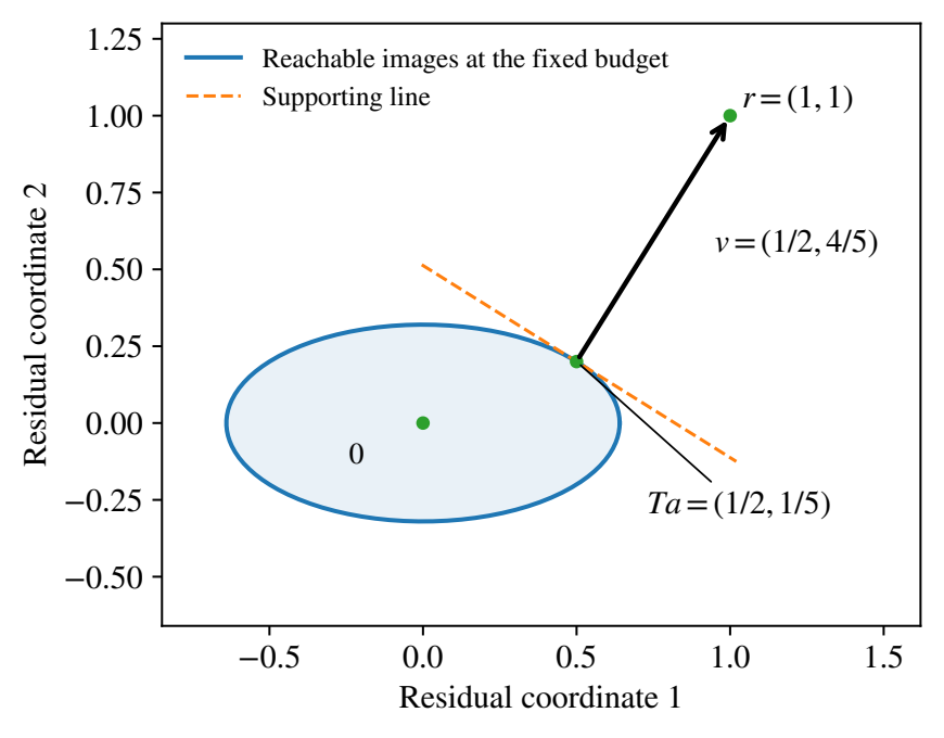
Take
Then \(T^*v=a\). At the budget \(M={\left\lVert a\right\rVert}=\sqrt{41}/10\), the normalized vector \(z=v/{\left\lVert v\right\rVert}\) gives
Consequently \(a\) is a globally optimal budgeted correction and \(\beta(M)=\sqrt{89}/10\). It is not necessary to compare it with a dense numerical grid of competing vectors. The supporting witness proves optimality over the entire ball.
28.4 How measurement and model uncertainty affect the budget
On this page · Permalink · Source line 131
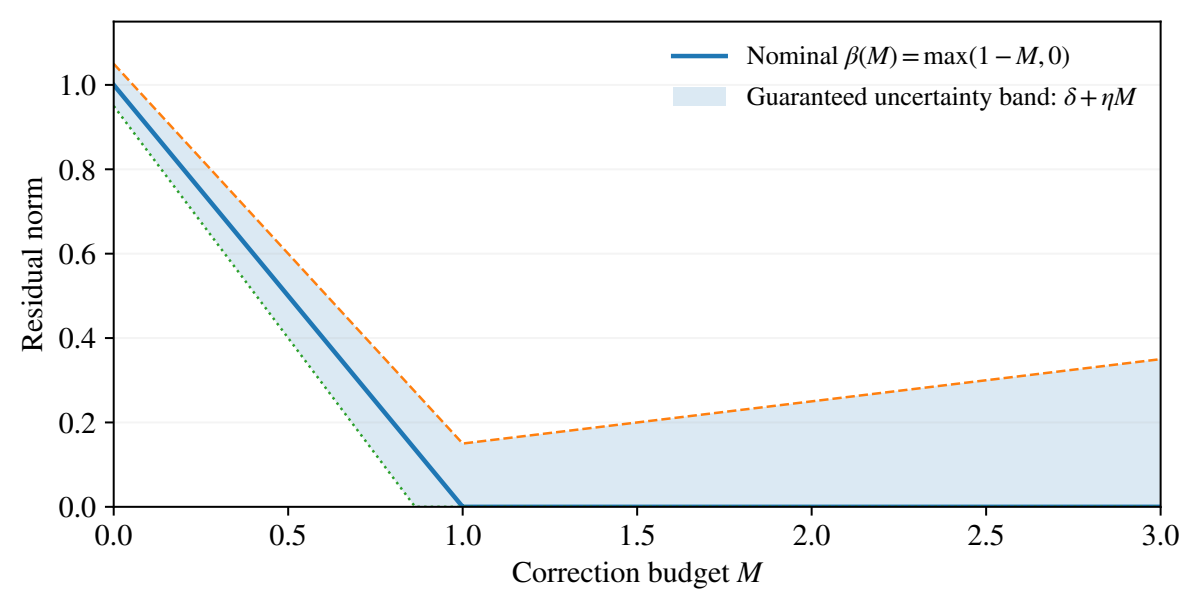
Theorem 28.3: A robust budget profile
Suppose the bounded linear map \(\widetilde T:H\to Y\) and the datum \(\widetilde r\in Y\) satisfy
For every \(M\ge0\),
In particular, for \({\left\lVert z\right\rVert}\le1\),
Proof
Fix a feasible correction \(a\). The two residual vectors have difference
whose norm is at most \(c=\delta+\eta M\). The reverse triangle inequality therefore gives both inequalities
The domain of feasible corrections is identical in the two problems. Taking the infimum of each inequality over that common domain yields
These are precisely the absolute-value bound. One could equivalently evaluate at the two attained minimizers, but no relation between those minimizers is needed.
For any admissible \(z\), Theorem 28.2 for the nominal problem gives
Combine this with the lower half of the preceding comparison. The result is a certificate against every correction in the original fixed ball, reduced by the explicit uncertainty allowance. If the correction space itself changed, the common-domain step would fail and this proof would no longer apply.
This estimate identifies a practical boundary of increasingly large corrections. A model error \(\eta\) is amplified by the correction budget even if the measured residual is tiny. The candidate-level inequality is
The theorem compares maps on one fixed correction space. It does not cover an uncertain preservation map whose kernel itself changes.