Finite observations and realized transformations

Proof

A finite-stage equality remains true after moving to a later stage. Indeed, if it holds on \(X_k\) and \(\ell\ge k\), precompose both sides with \(\rho^X_{k,\ell}\) and use the composite-restriction laws. Reflexivity uses \(k=\phi(n)\), symmetry reverses the equality, and transitivity moves two witnesses to their maximum. The shared middle presentation then cancels as a literal function on that common fiber. This proves an equivalence relation without referring to global points.

We check compatibility with composition with all indices displayed. Write \(f,f'\) with schedules \(\phi,\phi'\) and \(g,g'\) with schedules \(\psi,\psi'\). Fix an output level \(n\). Choose \(j\ge\psi(n),\psi'(n)\) with

Next choose \(k\ge\phi(j),\phi'(j)\) with

Monotonicity implies that \(k\) is also at least both composite input levels. Applying the naturality equations and then the two witness equations gives

This is the required equality on every element of \(X_k\). Thus composition descends to classes. The representative composition is associative because function composition and schedule composition are associative. The schedule \(n\mapsto n\) with identity coordinate maps gives both identity laws. Hence the quotient has the claimed category structure.

Finally, evaluate a witness equation at the \(k\)th coordinate of a coherent point \(x\). Its two restricted arguments become \(x_{\phi(n)}\) and \(x_{\psi(n)}\), proving equality of the realized outputs. Thus realization is well defined on the quotient. For a composite, direct evaluation gives

The identity law is equally coordinatewise. Joint determination of output points proves the functor laws.

Back to statement · Permalink · Source line 33

Proof

Realized equality follows from eventual equality by the preceding theorem, so only its converse remains. Suppose \(|f|=|g|\). Fix the output level \(n\), and let \(k=\max\{\phi(n),\psi(n)\}\). To prove equality of two maps defined on \(X_k\), fix an arbitrary element \(a\in X_k\). The assumed surjectivity of \(\operatorname{ev}_k\) supplies a coherent point \(x\) with \(x_k=a\). Equality of the two realized maps gives equality of their output coordinates:

Coherence of \(x\) rewrites this as

The index \(k\) was selected before \(a\), so this is one common finite-stage equality for all elements of \(X_k\). It is exactly the witness required by eventual equality at output \(n\). Repeating for each \(n\) proves faithfulness.

For the sufficient condition on bonding maps, fix \(k\) and \(a\in X_k\). Define coordinates below \(k\) by restriction of \(a\). At each later stage use surjectivity of the adjacent bonding map to choose a preimage of the coordinate already chosen. Recursion with classical choice constructs the upper tail. Adjacent equations hold by construction, and induction on the interval length gives every composite equation. This produces a point evaluating to \(a\). If a fiber is empty, the statement that each of its elements lifts is vacuous, as required by surjectivity onto that fiber. Without the projection-surjectivity assumption, equality on realizable inputs alone need not identify finite maps on values that never occur in a global point.

Back to statement · Permalink · Source line 77

Proof

For a reindexed map \((\phi,f)\), the formula \(|f|(x)_n=f_n(x_{\phi(n)})\) immediately supplies a finite-observation witness for each \(n\). Eventual equality does not affect the realized function by Theorem 7.1, so this defines a map from the quotient to the stated set of functions.

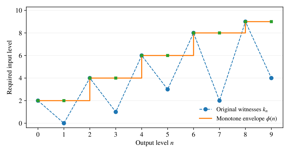
For surjectivity, let \(F\) be finitely observed. Choose one pair \((k_n,a_n)\) at each output level, satisfying \(F(x)_n=a_n(x_{k_n})\) for every coherent input. Define

The maximum is of a nonempty finite set. It gives a monotone schedule with \(k_n\le\phi(n)\). For every point \(x\), coherence in \(X\) gives

The remaining obligation is naturality on all finite states. Fix \(i\le j\) and \(u\in X_{\phi(j)}\). By surjectivity of that point projection, choose \(x\) with \(x_{\phi(j)}=u\). Equation (*) and output coherence yield

The state \(u\) was arbitrary. Hence the two finite-level functions are equal, which proves scheduled naturality. The resulting transport realizes \(F\) by (*).

Different witness choices can give different schedules and coordinate maps, but the realized function is still \(F\). By Theorem 7.2 these transports are eventually equal, so their quotient class is independent of all choices. The same faithfulness result says that two classes with equal realized functions are identical. We have proved both surjectivity and injectivity, including the well-definedness of the inverse choice construction. No bound on the growth of \(\phi\) follows from these quantifiers.

Back to statement · Permalink · Source line 113

Proof

Let \(s:X\to X_\theta\) be sampling, with schedule \(\theta\) and identity level maps. For recovery choose the least \(j(n)\) with \(n\le\theta(j(n))\). Unboundedness makes this set nonempty. Increasing \(n\) only strengthens the inequality, so \(j\) is monotone. The level map of \(r:X_\theta\to X\) is \(\rho^X_{n,\theta(j(n))}\). Composite restriction proves its naturality.

The composite \(rs:X\to X\) reads level \(\theta(j(n))\) and restricts to \(n\). At that very stage its map agrees with the identity transport after restriction from \(\theta(j(n))\) to \(n\). Thus \(rs\) is eventually equal to the identity.

For \(sr:X_\theta\to X_\theta\), the schedule at output \(n\) is \(j(\theta(n))\), and the level map is \(\rho^X_{\theta(n),\theta(j(\theta(n)))}\). Compare it with the identity at a sampled index

Restricting either route from level \(k\) of the sampled system gives the same original restriction \(\rho^X_{\theta(n),\theta(k)}\). This proves eventual equality even when \(\theta\) has repeated values. Hence the two classes are inverse isomorphisms, without requiring them to be literal inverse schedules.

Write \(s_X,r_X\) and \(s_Y,r_Y\) for the sampling and recovery isomorphisms of source and target. The asserted Hom map is

with inverse \([g]\mapsto r_Y[g]s_X\). Associativity and the two inverse equations cancel the inserted pairs, proving both round trips. Applying the realization functor transports these equations to point spaces, where sampling and recovery are the cofinal point equivalences already constructed. No norm invariance or surjectivity of source point projections is needed for this categorical conjugation argument.

Back to statement · Permalink · Source line 173