
Part V From approximation to exact realization
On this page · Permalink · Source line 1
A vanishing defect is a statement about measurements. A limiting realization also requires control of the candidate itself. This part follows the movement of approximate answers, the closure of admissible correction images, and the meaning of the ambient completion.
24 Exactification without a fixed contraction rate
On this page · Permalink · Source line 2
The constructed linear repair in Section 8 is a useful special case of a more general principle. One can prove convergence without one fixed contraction factor, without a linear update rule, and without a globally Lipschitz iteration. What must not be lost is control of the total movement.
24.1 The two limits that must be established
On this page · Permalink · Source line 5
Let \((M,{\operatorname{dist}})\) be a complete metric space. Let \(\omega:M\to[0,\infty)\) be a nonnegative residual function, and call a point exact when \(\omega(x)=0\). We regard \(\omega\) as a real-valued function when discussing continuity. Assume it is lower semicontinuous, so that every sublevel set \(\{x:\omega(x)\le a\}\) is closed.
For an approximation sequence \(f_n\), the statements
are different. The first concerns the observed discrepancy. The second concerns the mathematical candidate in the chosen metric. Neither implies the other without additional hypotheses.
Theorem 24.1: Summable movement gives exactification
Suppose \(b_n\ge0\), \(\sum_{n=0}^{\infty}b_n<\infty\), and
Then there is a limit \(x\in M\) satisfying
Proof
For integers \(m>n\), apply the triangle inequality successively along the finite chain \(f_n,f_{n+1},\ldots,f_m\). It gives
Given \(\varepsilon>0\), convergence of the nonnegative series supplies \(N\) for which the final tail is below \(\varepsilon\) whenever \(n\ge N\). Interchanging \(m,n\) when necessary proves the Cauchy condition for all pairs of indices at least \(N\). Completeness, not residual decay, is the hypothesis that now supplies a limit \(x\in M\).
Keep \(n\) fixed. The reverse triangle inequality says
Passing to the limit in the uniform tail bound proves the claimed distance certificate at that \(n\).
It remains to prove exactness of the limit. Fix \(\varepsilon>0\). Since \(\omega(f_m)\to0\), an entire tail of the sequence belongs to the sublevel set \(C_\varepsilon=\{z:\omega(z)\le\varepsilon\}\). Lower semicontinuity makes this set closed, so the limit of that tail belongs to it. Hence \(\omega(x)\le\varepsilon\) for every positive \(\varepsilon\). If \(\omega(x)>0\), choosing \(\varepsilon=\omega(x)/2\) contradicts this inequality. Since \(\omega\) is nonnegative, \(\omega(x)=0\). We have not used, or asserted, continuity of \(\omega\) or the stronger equality \(\omega(f_m)\to\omega(x)\) for arbitrary convergent inputs.
The formal theorem is slightly more general: it is stated in a complete pseudometric space. In a metric space the limit of this fixed sequence is unique. That does not mean different admissible approximation procedures select the same exact point.
24.2 Variable rates and a movement budget
On this page · Permalink · Source line 46
Let \(q_n,C_n\ge0\), and define the prefix product
Assume
Theorem 24.2: Variable-rate exactification
If \(Q_n\to0\) and \(\sum_n C_nQ_n<\infty\), then \((f_n)\) has an exact limit and
For constant \(q_n=q\in[0,1)\) and constant \(C_n=C\), the sharper restarted estimate is
Proof
The estimate \(\omega(f_n)\le Q_n\omega(f_0)\) follows by induction. At \(n=0\) it is equality. If it holds at \(n\), nonnegativity of \(q_n\) permits multiplication and gives
Because \(Q_n\to0\) and \(\omega(f_0)\) is a fixed finite number, the residual tends to zero. The movement assumption then gives
This is a summable nonnegative budget by the hypothesis on \(\sum C_nQ_n\). All assumptions of Theorem 24.1 now hold, and its tail certificate is exactly (24.2). If \(\omega(f_0)=0\), the same estimates make every step zero and every residual zero. No cancellation of that value was used.
For constant rates, the global estimate can be sharpened by restarting at the current index. Fix \(n\). A new induction on \(j\) gives
Sum the finite chain from \(n\) to \(n+m\), and then let \(m\to\infty\) using the already established limit. The geometric series equals \(1/(1-q)\), including \(q=0\), where its first term is one and all later terms vanish. This proves the restarted bound. The variable-rate proof itself requires only nonnegative \(q_n\), decay of their cumulative products, and summability of the movement weights. It does not insert an unstated upper bound \(q_n<1\) at each step.
The individual factors \(q_n\) need not all be below one. Temporary residual increases are permitted if the prefix products decay and the weighted movements remain summable. Conversely, a decaying product is not enough when its movement budget diverges.
24.3 A convergent path with no uniform geometric factor
On this page · Permalink · Source line 89
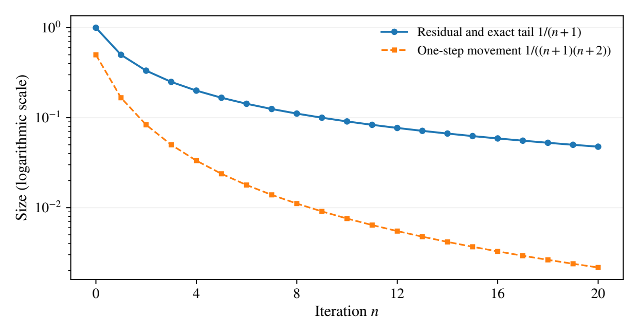
In \({\mathbb R}^2\) with the maximum norm, fix \(s\in{\mathbb R}\) and take
The protected coordinate is the first one. Direct calculation gives
No constant \(q<1\) bounds all the ratios \(q_n\), since they tend to one. Nevertheless
The limit is \((s,0)\), and the error bound is an equality. The model shows why the variable-rate theorem is not merely a rephrasing of a fixed geometric contraction.
24.4 Residual bursts can be compatible with convergence
On this page · Permalink · Source line 110
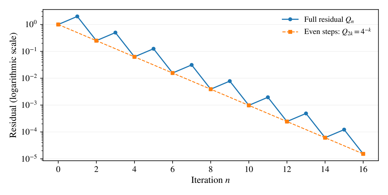
Set \(q_{2k}=2\), \(q_{2k+1}=1/8\). Then
For \(f_n=(s,Q_n)\), the residual doubles at the start of every pair of steps. Choose \(C_{2k}=1\) and \(C_{2k+1}=7/8\). These give equality in the movement bound, and
Thus \(f_n\to(s,0)\) despite infinitely many increases. Starting at an even index \(2k\), the remaining movement budget is \(\frac{11}{3}4^{-k}\). At an odd index \(2k+1\), it is \(\frac83 4^{-k}\). These bounds are larger than the actual distance because the path repeatedly moves away and returns.
24.5 Protected meaning survives a controlled limit
On this page · Permalink · Source line 125
Return to Banach and normed linear spaces, with continuous linear maps \(d:E\to R\) and \(p:E\to S\). Put \(\omega(f)={\left\lVert df\right\rVert}\). The residual is continuous, hence lower semicontinuous.
Proposition 24.3: Controlled paths kill the actual obstruction
Suppose \(E\) is complete, \({\left\lVert df_n\right\rVert}\to0\), \(p(f_n)=p(f_0)\), and \({\operatorname{dist}}(f_n,f_{n+1})\le b_n\) for a summable nonnegative budget. Then there is \(x\) with
and the constrained obstruction \([df_0]\in R/d(\ker p)\) vanishes.
Proof
The function \(f\mapsto{\left\lVert df\right\rVert}\) is continuous because \(d\) is bounded linear and the norm is continuous. It is therefore an admissible lower semicontinuous residual for Theorem 24.1. That theorem supplies a limit \(x\in E\), together with \({\left\lVert dx\right\rVert}=0\), which means \(dx=0\).
Continuity of \(p\) gives \(p(f_n)\to p(x)\). The left side is the constant sequence with value \(p(f_0)\). Uniqueness of limits in the normed target therefore gives \(p(x)=p(f_0)\). Define the actual vector \(a=f_0-x\). Linearity, rather than a closure argument, now yields
Thus \(a\in\ker p\) and \(df_0\in d(\ker p)\). Membership in this algebraic image is precisely what makes the class \([df_0]\) zero. Merely knowing membership in the closure of that image would not justify the same conclusion.
This proposition converts a controlled approximation argument into a statement about the algebraic quotient defined earlier. Merely showing that \(df_n\to0\) would not produce the admissible vector \(f_0-x\), because there might be no candidate limit \(x\).
24.6 When two repair paths select the same point
On this page · Permalink · Source line 147
Proposition 24.4: Path independence requires a comparison
Let \(f_n\to x\) and \(g_n\to y\) in a metric space. If
then \(x=y\). In contrast, exactness and preservation of a nonzero observable alone do not force a unique answer.
Proof
For each \(n\), the triangle inequality gives
Given any \(\varepsilon>0\), choose \(n\) large enough that the three terms on the right are each below \(\varepsilon/3\). Thus \({\operatorname{dist}}(x,y)\le\varepsilon\) for every positive \(\varepsilon\), so the distance is zero. The metric separation axiom gives \(x=y\). In a pseudometric space only zero distance would follow without an additional separation hypothesis.
For the negative assertion let \(E={\mathbb R}\times({\mathbb R}\times{\mathbb R})\), \(d(s,u,r)=r\), and \(p(s,u,r)=s\). Both \(x=(1,0,0)\) and \(y=(1,1,0)\) have zero defect and protected value one, but their middle coordinates differ. They are distinct points of the same feasible fiber. Constant sequences at those points meet exactness and preservation but not a vanishing comparison bound, so these conditions alone cannot imply path independence.
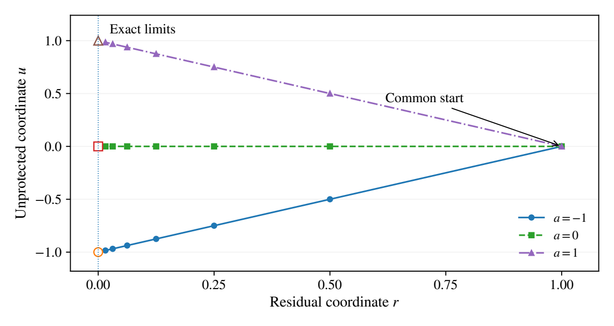
A stronger worked example uses actual convergent paths from the same initial input:
All paths begin at \((s,0,1)\), keep \(p=s\), and have residual \(2^{-n}\). Their maximum-norm movements are \(\frac12\max\{|a|,1\}2^{-n}\), so every path satisfies geometric exactification. Their limits are \((s,a,0)\). For different \(a,b\),
not zero. The missing uniqueness hypothesis is visible in the exact direction along which the paths separate.
24.7 Changing the sampling schedule does not preserve a rate
On this page · Permalink · Source line 178
A residual profile \(\eta_n\) indexed by resolution is not an iteration trajectory. Nevertheless a useful convergence property is invariant under a cofinal schedule when the profile is monotone.
Proposition 24.5: Cofinal sampling of a decreasing profile
Suppose \(\eta_n\ge0\) is nonincreasing and \(\phi:{\mathbb N}\to{\mathbb N}\) is monotone and unbounded. Then
Without the monotonicity of \(\eta\), the reverse implication can fail even for a cofinal schedule.
Proof
The schedule tends to infinity, so convergence of the full profile implies convergence of the sampled one. Conversely, choose a sampled value below any prescribed \(\varepsilon>0\). Every later index of the original profile has no larger value, by monotonicity. This proves convergence of the full profile.
For failure without monotonicity, take \(\eta_{2n}=0\), \(\eta_{2n+1}=1\), and \(\phi(n)=2n\). All sampled values vanish, but infinitely many original values equal one.
Even in the decreasing case, the numerical rate changes. The profile \(\eta_n=1/(n+1)\), sampled at \(\phi(n)=2^n-1\), becomes \(2^{-n}\). This is exponential decay in the number of observations, not a proof of a faster correction process at the original resolution scale.
24.8 Three hypotheses that cannot simply be dropped
On this page · Permalink · Source line 196
Summable movement. In maximum-norm \({\mathbb R}^3\), let
The first coordinate is protected and the residual is the last coordinate. It tends to zero with the same ratios as the polynomial example. The movement equals \(1/(n+1)\), however, and the unprotected coordinate diverges. Here \(C_n=1\), so \(\sum C_nQ_n\) is the divergent harmonic series. Residual decay and semantic preservation hold, but exactification of this path fails.
Completeness. In the metric space \((0,\infty)\), take \(f_n=1/(n+1)\) and \(\omega(x)=x\). The steps are summable and the residual tends to zero, but there is no limit in this space. Completing the space adds the missing zero. It is essential to say whether that completion belongs to the intended model.
Lower semicontinuity. In \({\mathbb R}\), define \(\omega(0)=1\) and \(\omega(x)=0\) for \(x\ne0\). The same positive sequence converges with summable movement and residual zero at every step, yet its limit is not exact. The zero sublevel set is not closed. This example isolates why convergence of measurements along a sequence must interact correctly with the ambient topology.