
27 A bounded repair budget can recover existence
On this page · Permalink · Source line 2
The preceding example does not merely lack a convergent iteration. It has no bounded family of increasingly accurate protected corrections. This suggests a converse question. If approximate corrections stay in one bounded region, does an exact answer exist?
For bounded linear equations in a Hilbert space, the answer is yes. This is an existence statement, not a claim that the given sequence converges in norm. A stronger conclusion becomes available when the candidates are the least norm solutions of nested finite constraint systems.
Do not conflate
The two bounded-realization theorems in this chapter have formal counterparts in the accompanying Lean project. The printed proof of bounded approximate feasibility uses the weak-subsequence lemma below, whose argument remains written background material. A formal counterpart does not by itself verify that printed proof route. The later budget, regularization-limit, noise, and solver-certificate results also have formal counterparts under their stated hypotheses, as do the explicit infinite diagonal estimates, asymptotic budget constant, and rounded noisy rate. Exact finite models have separate executable checks. The Hilbert and regularization background is classical [6]. No novelty is claimed for weak compactness or quadratic regularization.
27.1 The correction space is the protected kernel
On this page · Permalink · Source line 11
Let \(E,Y,Z\) be real Hilbert spaces, let \(d:E\to Y\) and \(p:E\to Z\) be bounded linear maps, and fix a raw candidate \(f\in E\). Write
The space \(H\) is a closed Hilbert subspace with the norm inherited from \(E\). An allowed correction is \(a\in H\), and its repaired candidate is \(f-a\). Thus
The protected exact problem is precisely \(Ta=r\). Restricting the domain before optimizing is important. A penalty on \({\left\lVert pa\right\rVert}\) would only discourage a change in the protected data, not prohibit it.
The adjoint below always means \(T^*:Y\to H\), taken with the inherited Hilbert metric on \(H\). In ambient coordinates this is the projection of \(d^*\) onto \(H\). A coordinate basis of \(\ker p\) need not be orthonormal. Its Gram matrix must then be included in any calculation of correction energy.
27.2 The compactness needed for the existence argument
On this page · Permalink · Source line 24
Lemma 27.1: Bounded sequences have weakly convergent subsequences
Every bounded sequence \((a_n)\) in a real Hilbert space has a subsequence converging weakly to some \(a\). Moreover,
Proof
Choose \(M\ge0\) with \({\left\lVert a_n\right\rVert}\le M\). If \(M=0\), every term is zero and the conclusion is immediate. Otherwise let \(H_0\) be the closed linear span of the countably many vectors \(a_n\). Finite rational linear combinations of those vectors form a countable dense set, so \(H_0\) is separable. Apply Gram–Schmidt to a countable dense sequence, omitting zero remainders. This gives either a finite orthonormal basis or a countable orthonormal sequence \((e_j)\) whose closed span is \(H_0\). The ambient Hilbert space itself need not be separable.
Each scalar sequence \(\langle a_n,e_j\rangle\) is bounded by \(M\). For the first coordinate choose a convergent subsequence, for the second choose a subsequence of that subsequence, and continue. Taking the \(k\)th term from the \(k\)th nested subsequence, with increasing original indices, yields \(a_{n_k}\) for which every fixed coordinate converges. Call the coordinate limits \(c_j\). In the finite-dimensional case only finitely many successive selections are required.
For each finite \(J\), Bessel's inequality and passage to the limit give
The nondecreasing partial sums are therefore bounded. Orthogonality makes the partial vector sums \(\sum_{j\le J}c_je_j\) Cauchy, so completeness defines \(a\in H_0\) with \({\left\lVert a\right\rVert}\le M\).
To verify weak convergence against \(h\in H_0\), choose a finite basis combination \(h_J\) close to \(h\). Then
For a prescribed tolerance, choose \(h_J\) first to control the second term and then \(k\) to control the first by finitely many coordinate limits. For a general \(h\) in the ambient space, write \(h=P_{H_0}h+h_\perp\). The orthogonal component pairs to zero with every \(a_{n_k}\) and with \(a\), reducing to the preceding case. This proves weak convergence against every test vector.
If \(a\ne0\), testing against \(a/{\left\lVert a\right\rVert}\) gives
The zero limit case follows from nonnegativity. Thus the lower-semicontinuity conclusion concerns the actual norms on the selected subsequence, not only the original bound \(M\).
Theorem 27.2: Bounded approximate feasibility
For a bounded linear map \(T:H\to Y\) between real Hilbert spaces and \(r\in Y\), the following are equivalent:
If all \({\left\lVert a_n\right\rVert}\le M\), an exact solution exists with norm at most \(M\).
Proof
If \(Ta=r\), the constant sequence \(a_n=a\) is bounded and has zero residual. For the converse, let \({\left\lVert a_n\right\rVert}\le M\) and \(Ta_n\to r\) in norm. By the preceding lemma there is a subsequence \(a_{n_k}\) converging weakly to \(a\in H\) with \({\left\lVert a\right\rVert}\le M\).
For every fixed \(y\in Y\), the adjoint identity and weak convergence give
The last limit equals \(\langle r,y\rangle\) because norm convergence implies convergence of each continuous pairing. Thus \(\langle Ta-r,y\rangle=0\) for every \(y\). Taking \(y=Ta-r\) gives \({\left\lVert Ta-r\right\rVert}^2=0\), hence \(Ta=r\).
This proof does not claim that \(Ta_{n_k}\) converges in norm merely because \(a_{n_k}\) converges weakly. Its norm convergence to \(r\) was a separate hypothesis. The boundedness of the candidate corrections is used to obtain a weakly convergent subsequence, and their accurate residuals are used to identify its image exactly. The bound \({\left\lVert a\right\rVert}\le M\) comes from weak lower semicontinuity, so the exact answer stays inside the same closed budget ball.
No closed range assumption appears. The theorem concerns a single datum and a bounded family of its corrections. Closed range is the stronger, uniform statement that every attainable datum admits a correction controlled by one residual gain.
An immediate contrapositive is useful. If \(r\in\overline{{\operatorname{ran}} T}\setminus{\operatorname{ran}} T\), then every sequence with \(Ta_n\to r\) satisfies \({\left\lVert a_n\right\rVert}\to\infty\). Otherwise infinitely many terms would lie in one bounded ball, contradicting the theorem along that subsequence. This recovers the escape mechanism of Section 26 without using the diagonal formula.
27.3 Existence does not make an arbitrary sequence converge strongly
On this page · Permalink · Source line 90
Take \(H=Y=\ell^2\) and \(Te_n=e_n/n\). The vectors \(a_n=e_n\) have norm one and satisfy \(Ta_n\to0\). An exact answer exists, namely zero. Yet \({\left\lVert e_n-e_m\right\rVert}=\sqrt2\) for \(n\ne m\), so no subsequence converges in norm.
The conclusion of Theorem 27.2 is the existence of a weak limit along a subsequence that solves the equation. It is not summable movement, a strong convergence rate, or a selection rule for the original candidates. The minimum correction for the zero datum is zero, which this particular sequence never approaches in norm.
27.4 Minimum energy finite repairs do converge strongly
On this page · Permalink · Source line 95
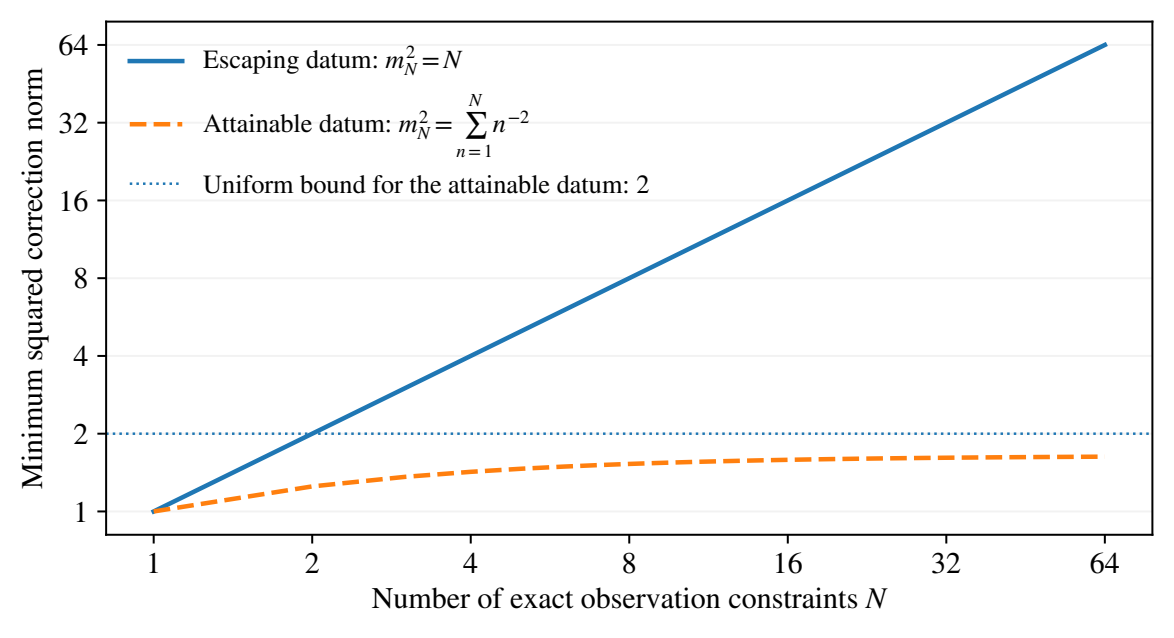
Suppose now that \(A_1\supseteq A_2\supseteq\cdots\) are nonempty closed affine subsets of a real Hilbert correction space \(H\). A typical \(A_n\) consists of corrections satisfying the first \(n\) bounded linear observation equations. The sets are affine because the equations are linear, and closed because the observations are continuous.
Let \(a_n\) be the unique point of \(A_n\) nearest to zero, and put \(m_n={\left\lVert a_n\right\rVert}\). The Hilbert projection theorem supplies these points. It can also be proved directly: a sequence approaching the minimum norm is Cauchy by the parallelogram identity, its limit belongs to the closed convex set, and the same identity gives uniqueness.
Theorem 27.3: A uniform finite budget yields a strong realization
For the nested affine sets above, \(m_n\) is nondecreasing, and for \(m\ge n\),
Their intersection is nonempty if and only if \(\sup_n m_n<\infty\). In that case \(a_n\) converges in norm to the unique least norm point \(a_*\in\bigcap_n A_n\), with
If the intersection is empty, then \(m_n\to\infty\).
Proof
The nearest-point theorem for nonempty closed convex subsets of a Hilbert space, proved in Appendix E, supplies \(a_n\). Write \(A_n=a_n+L_n\), where \(L_n\) is its closed direction subspace. For \(\ell\in L_n\) and every real \(t\), the vector \(a_n+t\ell\) belongs to \(A_n\). Minimality implies
Allowing both signs of arbitrarily small \(t\) forces \(\langle a_n,\ell\rangle=0\).
If \(m\ge n\), nesting gives \(a_m\in A_n\), so \(a_m-a_n\in L_n\). Expanding its norm therefore gives
This is the exact energy identity. It also makes \(m_n^2\) nondecreasing.
Suppose these energies are bounded, and let \(L=\lim_n m_n^2\). Given \(\epsilon>0\), choose \(N\) with \(L-m_N^2<\epsilon^2\). For \(m\ge n\ge N\),
Thus \((a_n)\) is Cauchy and has a norm limit \(a_*\). For each fixed \(n\), all terms from that index onward belong to the closed set \(A_n\), so \(a_*\in A_n\). This places \(a_*\) in their entire intersection.
If \(a\) lies in the intersection, then \({\left\lVert a\right\rVert}\ge{\left\lVert a_n\right\rVert}\) for every \(n\). Norm continuity gives \({\left\lVert a\right\rVert}\ge{\left\lVert a_*\right\rVert}\). Uniqueness follows from the nearest-point theorem applied to the intersection, which is closed and convex and now known to be nonempty. Alternatively, the midpoint of two different minimizers would have strictly smaller norm by the parallelogram identity. Taking \(m\to\infty\) in the finite energy identity yields
Conversely, any element of the intersection bounds every minimum norm from above. Therefore an empty intersection forces the nondecreasing sequence \(m_n\) to be unbounded. A nondecreasing unbounded nonnegative sequence tends to infinity, giving the last conclusion.
The finite answers need not extend one another coordinate by coordinate. Their shared feature is minimum energy in one common ambient Hilbert space. This is the extra geometry that forces their differences to be orthogonal to the earlier minimizers.
For the attainable diagonal datum \(r_n=1/n^2\) under \(Tu=(u_n/n)\), with \(n\ge1\), the first \(N\) equations force correction coordinate \(n\) to equal \(1/n\) for \(n\le N\). Their minimum energy completion is zero beyond \(N\), and
These corrections converge strongly to \((1/n)\). For the escaping datum \(r_n=1/n\), the corresponding energy is \(m_N^2=N\). Every finite equation is again solved, but the budget test now rules out an ambient solution.
How to read the result
Finite consistency is not enough by itself. For nested closed affine problems in one Hilbert space, a uniform bound on the minimum correction norms is exactly what upgrades finite feasibility to ambient feasibility. This is a datum-specific test, not a uniform inverse bound for the operator.