
Part IV The geometry of exact realization
On this page · Permalink · Source line 1
A categorical space of realizations does not come with a numerical distance by default. In a declared linear model, the compatibility equations become a bounded operator. Closed range, holonomy, and conditioning then determine what small residuals actually guarantee.
17 Graph views, holonomy, and reconstruction
On this page · Permalink · Source line 2
17.1 Actual transports on a finite graph
On this page · Permalink · Source line 3
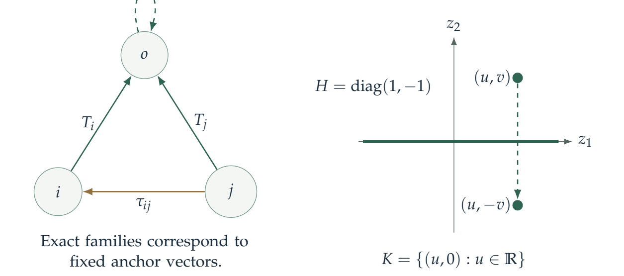
Let a finite connected simple graph have vertex set \(V\), root \(o\), and a chosen route \(p_i:o\to i\) for every vertex, with the route at \(o\) empty. Use a common real normed fiber \(H\). An inverse consistent connection assigns continuous linear equivalences \(\tau_{ij}\), with \(\tau_{ji}=\tau_{ij}^{-1}\). Our convention is that \(\tau_{ij}\) carries the value at \(j\) into the coordinates at \(i\).
The candidate and residual spaces are finite products with maximum norms:
Both orientations of an edge are retained. If \(M\) bounds the norms of all measured edge maps, then \({\left\lVert d\right\rVert}\le M+1\). The empty edge case has the usual zero residual.
Distinct walks are retained as arrows of the view category. The product along a walk \(q=(i_0,\ldots,i_m)\) is
Concatenation gives the restriction composition law. An exact vertex family defines a coherent walk-view section, and a coherent walk-view section satisfies every edge equation. Thus this graph construction returns to the original ambient realization type rather than creating a disconnected numerical model.
17.2 Transported residuals and path gains
On this page · Permalink · Source line 20
Proposition 17.1: The path telescope
For a walk \(q=(i_0,\ldots,i_m)\),
The empty prefix is the identity. If \(\gamma(q)\) is the sum of the products of preceding edge norms, then
Proof
Write \(U_0=I\) and \(U_k=\tau_{i_0i_1}\cdots\tau_{i_{k-1}i_k}\) for \(1\le k\le m\). The transport convention makes every \(U_k\) a map from the fiber at \(i_k\) to that at \(i_0\). Since \(U_{k+1}=U_k\tau_{i_ki_{k+1}}\), the \(k\)-th transported defect is
Summing over \(k=0,\ldots,m-1\) cancels each interior value once with each sign. The remaining terms are \(U_mx_{i_m}-U_0x_{i_0}=T_qx_{i_m}-x_{i_0}\), proving the identity with its actual ordered products. For an empty walk both sides are zero.
The triangle inequality and the operator norm bound now give
The bracket is \(\gamma(q)\), with the empty product equal to one. Repeated vertices or edges do not affect the cancellation. Reordering the edge maps would, in general, invalidate it.
For isometric maps, \(\gamma(q)\le|q|\). For arbitrary bounded equivalences, route length cannot replace the amplification gain. Reversing a route can have a different gain, even though its transport is the inverse map.
17.3 Holonomy is the remaining exactness condition
On this page · Permalink · Source line 52
Write \(T_i=T_{p_i}\). Reconstruction from a proposed root value is
For each directed edge define the root loop operator
Each \(K_{ij}\) is the transport around an actual rooted loop. No flatness assumption has been made.
Theorem 17.2: Holonomy classification
Evaluation at the root and reconstruction give an equivalence
A root value extends to an exact vertex family precisely when it lies in \(K\), and that extension is unique. The space \(K\) is independent of the chosen routes. Reconstruction is route independent on \(K\).
Proof
Every \(T_i\) is a continuous linear equivalence, being a finite ordered composition of such maps. Reconstruction is therefore well defined. For an edge \((i,j)\), apply \(T_i\) to its defect:
Because \(T_i\) is injective, that edge defect is zero if and only if the corresponding root loop fixes \(z\). Thus \(dR_pz=0\) holds exactly for \(z\in K\). The root route is empty, so \((R_pz)_o=z\).
Conversely, let \(x\in\ker d\). The path telescope along \(p_i\) has all zero summands, hence \(T_ix_i=x_o\) for every vertex. Applying \(T_i^{-1}\) gives \(x_i=T_i^{-1}x_o\), so \(x=R_p(x_o)\). The first part then places \(x_o\) in \(K\). We have proved both inverse equations and uniqueness of an exact extension of a root value.
The maps are linear. On the finite vertex product,
These bounds also hold on the subspaces \(K\) and \(\ker d\), proving continuity of both directions. No completeness is needed for these finite bounds.
For route independence, the proved equivalence identifies \(K\) with the image of root evaluation from the intrinsically defined space \(\ker d\). That image does not refer to any chosen routes, so every route system yields the same \(K\). For \(z\in K\), reconstruction using either system is an exact family with root \(z\), and uniqueness makes the families equal. For \(z\notin K\), this uniqueness argument does not assert equality of the two generally inconsistent reconstructed families.
With isometric transports the equivalence is an isometry for the vertex maximum norm, because every reconstructed coordinate has the root norm. With general bounded equivalences, it need not be an isometry.
17.4 Prescribed observations remain visible
On this page · Permalink · Source line 95
If a prescribed vertex set \(U\) contains \(o\), a candidate \(x\) has an exact repair preserving \(x|_U\) precisely when
Necessity follows from the classification. Sufficiency is the reconstructed family itself. The source identifies this criterion with the earlier obstruction class in \(R/d(\ker p_U)\). A graph seed test is therefore an instance of the same protected correction problem, not a replacement for it.
18 Closed range is the stability boundary
On this page · Permalink · Source line 102
18.1 Projection exists before a residual estimate
On this page · Permalink · Source line 103
Let \(E\) be a real Hilbert space and \(R\) a real Banach space. Let \(D:E\to R\) be continuous linear. The kernel \(K=\ker D\) is closed, so its orthogonal projection \(q=P_K\) exists [4].
Proposition 18.1: Exact orthogonal repair
For every \(x\in E\),
and \(qx\) is the unique closest point to \(x\) in \(K\).
Proof
Boundedness of \(D\) makes \(K=\ker D\) closed. Lemma E.1 constructs \(q=P_K\) and gives the orthogonal decomposition \(x=qx+(x-qx)\). The first term belongs to \(K\), so \(Dqx=0\). Projection fixes every point of \(K\), giving \(q(qx)=qx\).
Pythagoras applied to that decomposition gives \({\left\lVert x\right\rVert}^2={\left\lVert qx\right\rVert}^2+{\left\lVert x-qx\right\rVert}^2\), hence \({\left\lVert qx\right\rVert}\le{\left\lVert x\right\rVert}\). For any \(y\in K\), the vector \(qx-y\) lies in \(K\), whereas \(x-qx\) lies in its orthogonal complement. Consequently
Equality holds only when \({\left\lVert qx-y\right\rVert}=0\), or \(y=qx\). This proves nearest-point uniqueness without any closedness assumption on \({\operatorname{ran}} D\). Closedness of the kernel and of the range serve different purposes.
No closed range assumption on \(D\) is needed for this projection. Such an assumption enters when the size of the residual is asked to control the distance to the exact space.
Theorem 18.2: Closed range and quantitative exactness
The following are equivalent:
\({\operatorname{ran}} D\) is closed.
There is \(C\ge0\) with \({\left\lVert x-qx\right\rVert}\le C{\left\lVert Dx\right\rVert}\) for all \(x\).
There is \(C\ge0\) such that every \(x\) has some exact \(y\) with \({\left\lVert x-y\right\rVert}\le C{\left\lVert Dx\right\rVert}\).
When the range is closed, the least admissible constant is the operator norm of the inverse of \(D:K^\perp\to{\operatorname{ran}} D\). In the zero operator case that inverse has zero dimensional domain and its norm is zero.
Proof
Let \(K=\ker D\) and \(K^\perp\) carry the induced Hilbert norm. Define \(D_\perp u=Du\), but regard its target as \({\operatorname{ran}} D\) with the norm inherited from \(R\). It is injective: \(Du=0\) puts \(u\) in both \(K\) and \(K^\perp\), so \(u=0\). It is surjective onto that target: if \(r=Dx\), then \(u=x-qx\in K^\perp\) and \(Du=Dx=r\). Thus it is a bounded linear bijection before any continuity of its inverse is claimed.
Suppose first that the range is closed. Because \(R\) is Banach, \({\operatorname{ran}} D\) is then Banach. The domain \(K^\perp\) is also complete. The bounded inverse theorem, proved in Appendix E, gives a bounded inverse \(A=D_\perp^{-1}\). Applying it to \(Dx=D(x-qx)\) yields
Hence condition 2 holds. If any \(C\ge0\) satisfies condition 2, then for every \(r\in{\operatorname{ran}} D\) apply it to \(u=Ar\in K^\perp\). Since \(qu=0\), it gives \({\left\lVert Ar\right\rVert}\le C{\left\lVert r\right\rVert}\). Taking the operator norm proves \({\left\lVert A\right\rVert}\le C\). This establishes the least constant, not just a sufficient one. If \(D=0\), both \(K^\perp\) and the range are zero spaces and \({\left\lVert A\right\rVert}=0\).
Now assume condition 2. To prove closedness, take an arbitrary sequence \(r_n\in{\operatorname{ran}} D\) with \(r_n\to r\) in \(R\). Choose \(x_n\) with \(Dx_n=r_n\) and put \(u_n=x_n-qx_n\). Then \(u_n\in K^\perp\) and \(Du_n=r_n\). Applying the estimate to \(u_n-u_m\) gives
Thus \((u_n)\) is Cauchy in the complete space \(K^\perp\). Let its limit be \(u\). Continuity gives \(Du=\lim_n r_n=r\), so \(r\in{\operatorname{ran}} D\). In a normed space, a set containing the limits of all its convergent sequences is closed. This proves condition 1 without presupposing that the initially unbounded inverse is continuous.
Condition 2 implies condition 3 by choosing \(y=qx\). Conversely, if condition 3 supplies an exact \(y\) for a given \(x\), the nearest-point property of \(qx\) gives
The same \(C\) works for all \(x\), proving condition 2. This last implication does not require the selected answers \(y\) to depend linearly or continuously on \(x\).
The last equivalence is important. A nonlinear choice of exact answers cannot bypass the failure of a uniform residual bound. Failure of closed range is not merely a defect of one selected projection algorithm.
18.2 A small residual far from exactness
On this page · Permalink · Source line 158
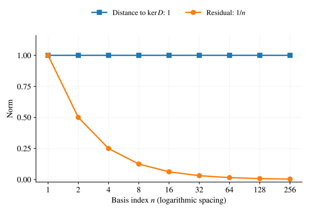
On \(\ell^2({\mathbb N})\), index the standard basis from one and define \(De_n=n^{-1}e_n\). The map is bounded and injective, so its exact space is zero. Yet
No finite \(C\) can bound \({\operatorname{dist}}(e_n,\ker D)\) by \(C{\left\lVert De_n\right\rVert}\). The range is not closed. For example finite truncations of \((1/n)_{n\ge1}\) belong to the range and converge in \(\ell^2\), but a preimage of the limit would be the constant sequence, which does not belong to \(\ell^2\).
This diagonal model is formalized on the infinite Hilbert space used in Section 30. In the namespace KomorebiSpace.DiagonalRegularization, T_not_closed_range applies the general obstruction theorem to actual unit coordinate vectors. The declaration w_mem_closure_not_range proves that the displayed limiting datum belongs to the closure of the range but not to the range itself. Formal coordinate \(j\) represents the printed coordinate \(n=j+1\).
18.3 Norm zero versus algebraic zero
On this page · Permalink · Source line 169
If an additive correction image is not closed, distance to that image can vanish without actual membership. Thus an infimum of residual error can be zero while the exact protected correction is unattained. The algebraic obstruction quotient and its possible seminorm answer different questions. One must identify a closed image, compactness condition, or other attainment principle before replacing one question by the other.
18.4 Stable repair with protected data
On this page · Permalink · Source line 172
The preceding orthogonal projection does not generally preserve a separately declared observable. To join the analytic theory to Section 4, let \(p:E\to S\) be continuous linear into a normed space. Define
The closed subspace \(M\) inherits its Hilbert structure from \(E\). A candidate \(x\) is feasible for protected repair when an exact \(y\) with \(p(y)=p(x)\) exists. The algebraic criterion is still \(Dx\in{\operatorname{ran}} B\).
Theorem 18.3: Nearest feasible protected repair
Every feasible \(x\) has a unique closest exact answer \(y_*\) preserving \(p(x)\). Its correction \(h_*=x-y_*\) is the unique vector in the orthogonal complement of \(\ker B\) inside \(M\) satisfying \(Bh_*=Dx\). For every other feasible answer \(y\),
Moreover, the following conditions are equivalent:
When these conditions hold, the least nonnegative constant is the transverse inverse norm of \(B\), including the zero-range case.
Proof
Feasibility gives some \(h_0=x-y_0\in M\) with \(Bh_0=Dx\). Conversely, every \(h\in M\) satisfying \(Bh=Dx\) produces an exact protected answer \(y=x-h\). Thus the answer problem and the correction problem are equivalent, with correction set
This is a nonempty closed affine subset of the Hilbert space \(M\). Closedness of \(\ker B\) follows from continuity of \(B\), independently of whether its image is closed.
Let \(k_0=P^M_{\ker B}h_0\) and \(h_*=h_0-k_0\). Then \(Bh_*=Bh_0=Dx\) and \(h_*\perp\ker B\) in \(M\). If a different initial correction is chosen, it differs from \(h_0\) by an element of \(\ker B\). Its orthogonal-complement component is therefore again \(h_*\). This proves that the construction is independent of the feasibility witness.
Every other correction can be written uniquely as \(h_*+k\) with \(k\in\ker B\). Orthogonality gives
Writing \(y_*=x-h_*\) and \(y=x-h_*-k\), we have \(x-y=h_*+k\) and \(y_*-y=k\). Substitution proves the stated Pythagorean identity. Its last term vanishes only when \(y=y_*\), establishing the unique closest answer.
If \({\operatorname{ran}} B\) is closed, Theorem 18.2 applied on \(M\) gives a bounded inverse of \(B\) on \((\ker B)^{\perp_M}\). The vector \(h_*\) is exactly that inverse applied to \(Dx\), so its norm obeys the required bound.
For the converse, suppose the bound holds for every feasible raw candidate. Every \(x\in M\) is feasible, because \(y=0\) has \(Dy=0\) and \(py=px=0\). Its closest protected exact answer is \(P^M_{\ker B}x\). Thus the assumed estimate reduces on \(M\) to
Theorem 18.2 forces \({\operatorname{ran}} B\) to be closed. The same restriction also proves that no smaller nonnegative constant than the transverse inverse norm can work. If the range is zero, feasible candidates are already exact under permitted correction and the least correction is zero, so the optimal gain is zero.
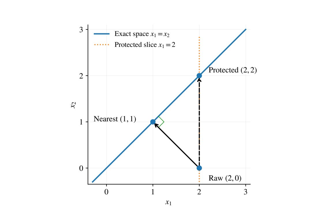
The relevant stability boundary is therefore \(D(\ker p)\), not automatically \(D(E)\). Restricting permitted changes can turn a well-conditioned unconstrained problem into an obstructed or poorly conditioned protected one. The nearest protected answer is generally not \(P_{\ker D}x\).
For \(D(x_1,x_2,x_3)=x_1-x_2\), \(p(x)=(x_1,x_3)\), and \(x=(2,0,5)\), the ordinary orthogonal answer is \((1,1,5)\). The protected answer is \((2,2,5)\). The respective squared errors are two and four. Both have zero residual, but only the latter preserves the declared data. The theorem is formalized in ProtectedHilbertRepair.lean, using the actual operator on \(\ker p\). The displayed three-coordinate values are an illustrative calculation, not a separate universal algorithm.
19 Holonomy repair and transport amplification
On this page · Permalink · Source line 223
19.1 An orthogonal anchor, not a global least squares answer
On this page · Permalink · Source line 224
Return to the graph model with a real Hilbert fiber. The root residual is
Let \(q=P_K\), and define
This is always exact, fixes exact families, and is idempotent. It is the unique exact family preserving the feasible component \(qx_o\) of the anchor. Its orthogonality is on the anchor fiber. The vertex and edge norms are still maximum norms.
For example on a two-vertex identity connection, \((0,2)\) with root value zero is repaired to \((0,0)\). The constant family \((1,1)\) is closer in the maximum norm, but it does not preserve the anchor. The operator \(P\) is not being claimed to be a global nearest-point projection in that norm.
19.2 Every factor in the bound has a meaning
On this page · Permalink · Source line 237
Define the route gain
using reverse routes so that the error is measured in each destination view. The path telescope gives
Let \(N_p\) be the residual normalization \((N_pr)_{ij}=T_ir_{ij}\). The exact identity \(\mathcal H=N_pdR_p\) implies
Theorem 19.1: Amplified holonomy repair
If \({\operatorname{ran}}\mathcal H\) is closed and \(\kappa\) is its transverse inverse gain, then
The range condition is necessary for the existence of any uniform bound of distance to an exact family by \({\left\lVert dx\right\rVert}_\infty\). It is automatic for a fixed finite dimensional fiber, but not uniformly quantitative across all connections.
Proof
First quantify the residual seen at the root. The identity \(\mathcal H=N_pdR_p\), applied to \(x_o\), gives
Closed range of \(\mathcal H\) lets Theorem 18.2 control the anchor correction by \({\left\lVert x_o-qx_o\right\rVert}\le\kappa{\left\lVert\mathcal H(x_o)\right\rVert}_\infty\). Insert the uncorrected reconstruction between \(x\) and \(Px=R_pqx_o\):
Substituting the two preceding bounds yields (19.1). The finite maximum-norm residual product is a Banach space because its fiber is Hilbert, so the target completeness needed in Theorem 18.2 is available.
For necessity, suppose a constant \(C\) satisfies \({\operatorname{dist}}(w,\ker d)\le C{\left\lVert dw\right\rVert}_\infty\) for every vertex family \(w\). Fix \(z\in K^\perp\) and take \(w=R_pz\). Every exact family \(e\) has \(e_o\in K\), and root evaluation has norm at most one. Therefore
Taking the infimum over \(e\in\ker d\) is legitimate without assuming that this global nearest point is attained. It gives
Here \(N_p\) is a continuous linear equivalence on the finite edge product because every component \(T_i\) is one. For a general root vector, remove its projection onto \(K\); this leaves the same \(\mathcal H\)-image and puts it in \(K^\perp\). Thus the displayed estimate is a uniform residual bound of the kind in Theorem 18.2, which forces \({\operatorname{ran}}\mathcal H\) to be closed. A finite-dimensional fiber makes that image finite dimensional and hence closed. It does not give a uniform numerical value of the inverse gain across different connections.
For isometric transports, one can use \({\left\lVert R_p\right\rVert}\le1\), \({\left\lVert N_p\right\rVert}\le1\), \({\left\lVert d\right\rVert}\le2\), and \(A_p\le r\), where \(r\) is the route radius. The bound reduces to
The exact repair is route independent for a fixed root and inner product. A chosen upper bound involving route gains need not have the same numerical value for different routes.
19.3 Flatness does not remove amplification
On this page · Permalink · Source line 298
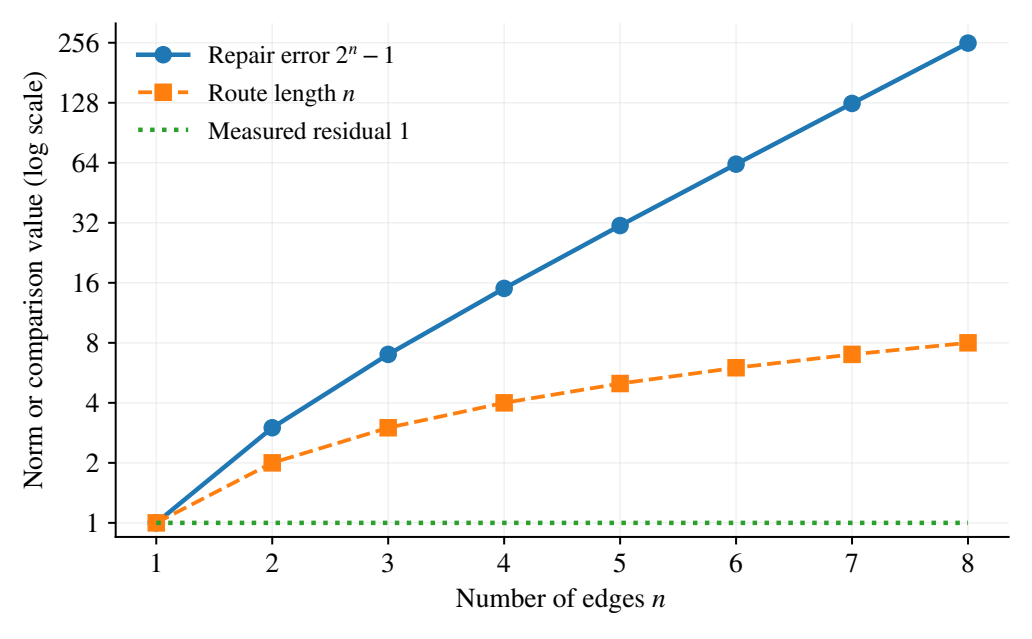
Consider a scalar chain with \(n+1\) vertices, where \(n\ge1\), and coordinates \(e_i(z)=2^iz\). Set \(\tau_{ij}=e_ie_j^{-1}\). This connection is flat, but reverse transport along one edge multiplies norms by two. Let
The family \(y\) is exact and preserves \(x_o=7\). On a forward edge the residual of \(x\) is \(1/2\), and on its reverse it is \(-1\). Thus
For \(n\ge2\), a route length bound of \(n\) fails. This is amplification with trivial holonomy, distinct from poor conditioning of the fixed space of a nearly trivial loop.
19.4 Small holonomy can still be poorly conditioned
On this page · Permalink · Source line 312
In \({\mathbb R}^2\), the rational rotation
satisfies
For \(t\ne0\) its fixed space is zero and its residual gain is \(\sqrt{1+t^2}/(2|t|)\), which diverges as \(t\to0\). At \(t=0\), the entire fiber is fixed. Therefore small loop discrepancy does not supply a uniform stable realization estimate. The fixed directions and their conditioning must be analyzed together.
20 Quantitative descent in a common Hilbert model
On this page · Permalink · Source line 324
20.1 Local exactness and matching are separate operators
On this page · Permalink · Source line 325
Let \(E\) be a real Hilbert space of raw local candidates. Let \(D:E\to R\) and \(C:E\to Y\) be continuous linear maps into Banach spaces, measuring local equation defects and overlap mismatch, respectively. Put
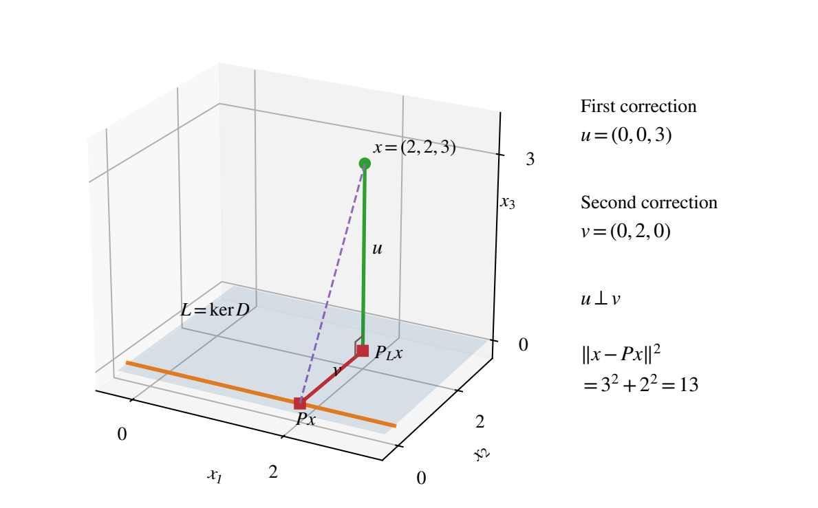
The exact matched families form \(M\). First project to \(L\), then project inside \(L\) to \(\ker B\). Denote the resulting map by \(P\).
Theorem 20.1: The two-stage repair is the joint projection
The operator \(P\) is the orthogonal projection onto \(M\), equivalently onto the kernel of \(\Delta=(D,C)\). If \(u=x-P_Lx\) and \(v=P_Lx-Px\), then
Proof
The subspace \(L=\ker D\) is closed, hence Hilbert with the inherited inner product. The restriction \(B=C|_L\) is continuous, so its kernel is a closed subspace of \(L\). Under the inclusion into \(E\), this kernel is exactly \(M=L\cap\ker C\). Thus both projections used to define \(P\) exist.
For an input \(x\), write \(\ell=P_Lx\) and let \(Px\) be the projection of \(\ell\) onto \(\ker B\) inside \(L\). Then \(Px\in M\), \(u=x-\ell\in L^\perp\), and \(v=\ell-Px\in L\) is orthogonal to \(M\). Since \(M\subseteq L\), the vector \(u\) is also orthogonal to \(M\). Their sum \(x-Px=u+v\) is therefore orthogonal to \(M\). A vector in \(M\) with that error is the unique orthogonal projection of \(x\), so \(P=P_M\).
The two errors themselves are orthogonal because \(u\in L^\perp\) and \(v\in L\). Expanding the squared norm of their sum gives \({\left\lVert x-Px\right\rVert}^2={\left\lVert u\right\rVert}^2+{\left\lVert v\right\rVert}^2\). Finally \(\ker(D,C)=\ker D\cap\ker C=M\), so this is also the projection onto the kernel of the joint defect. The proof uses a second projection inside \(L\). Replacing it by the ambient projection onto \(\ker C\) would invalidate the membership step and need not preserve local exactness.
This identity does not require the local and overlap operators to commute. The second projection is taken in the already exact subspace, not in the whole raw space without restriction.
For a concrete failure of the unrestricted procedure, take \(L=\{(a,0)\}\) and \(\ker C=\{(a,a)\}\) in \({\mathbb R}^2\). Their intersection is zero. Starting from \((1,0)\), projection to \(L\) does nothing, while subsequent projection to \(\ker C\) gives \((1/2,1/2)\), which is no longer in \(L\). The restricted second stage instead gives the correct joint answer zero.
20.2 A stable repair requires a stable matching problem
On this page · Permalink · Source line 353
Suppose \({\operatorname{ran}} D\) and \({\operatorname{ran}} B\) are closed, with residual gains \(a,b\). Then
Therefore
The Pythagorean identity gives the sharper estimate
For the maximum norm on \(R\times Y\), two sufficient gains are therefore
The inequality follows from \(\sqrt{u^2+v^2}\le u+v\) for nonnegative \(u,v\). The formal interface supplies the sum-type gain \(G_1\), while its squared-error theorem also yields \(G_2\). Neither is claimed to be the least joint gain. In either bound, \({\left\lVert C\right\rVert}\) may be replaced by any certified bound on \(C\) restricted to \((\ker D)^\perp\).
Theorem 20.2: Closed range for the joint defect
Assume \({\operatorname{ran}} D\) is closed. Then
Under either condition, a finite joint residual-to-repair bound exists.
Proof
Suppose the range of the joint map is closed. To test closedness of \({\operatorname{ran}} B\), take a sequence \(Bk_n\to y\) with \(k_n\in\ker D\). The joint images are
Closedness supplies \(x\in E\) with \((Dx,Cx)=(0,y)\). The first coordinate gives \(x\in\ker D\), and the second gives \(Bx=y\). Hence the matching range is closed. This direction did not require closedness of \({\operatorname{ran}} D\).
For the reverse direction, assume both \({\operatorname{ran}} D\) and \({\operatorname{ran}} B\) are closed, and take joint images converging to \((r,y)\). Thus \(Dx_n\to r\) and \(Cx_n\to y\). Decompose each input orthogonally as
Because \(r\in{\operatorname{ran}} D\) and the transverse inverse \(A\) of \(D\) is bounded by Theorem 18.2, the first components determine
Continuity of \(C\) now gives
Closedness of \({\operatorname{ran}} B\) supplies \(k\in\ker D\) with \(Bk=y-Cu\). There is no need for the sequence \(k_n\) itself to converge. The single vector \(u+k\) satisfies
Thus the joint limit lies in the joint range, proving closedness. The target product is Banach under its maximum norm, so Theorem 18.2 applies to the joint map and gives a finite repair gain. The earlier two-stage estimate supplies an explicit, though not necessarily least, value.
This Hilbert model is a quantitative counterpart of gluing, but it is not a norm on an arbitrary categorical stack. It starts from a fixed raw candidate space, fixed norms, and actual local and overlap operators. Changing those choices requires its own comparison.
21 Controlled motion of exact spaces
On this page · Permalink · Source line 418
21.1 A two-sided condition number theorem
On this page · Permalink · Source line 419
Let \(D,D':E\to R\) be continuous linear maps from a real Hilbert space to the same normed target. Write \(q=P_{\ker D}\), \(q'=P_{\ker D'}\). Suppose
and \({\left\lVert D-D'\right\rVert}\le\varepsilon\).
Theorem 21.1: Motion of the exact projector
Without either kernel inclusion as a hypothesis,
In particular a uniform residual gain \(M\) makes \(D\mapsto P_{\ker D}\) \(M\)-Lipschitz on the class of operators carrying that gain.
Proof
For \(z\in\ker D'\), the old residual bound gives
Interchanging the roles gives
We need a dual form of (*). For \(v\in(\ker D')^\perp\) and any \(y\in E\), self-adjointness of \(q\) and \(v=(I-q')v\) give
The Hilbert norm equals the supremum of these pairings on the unit ball, so \({\left\lVert qv\right\rVert}\le C'\varepsilon{\left\lVert v\right\rVert}\). This proves the precise restriction estimate needed on \((I-q')x\), not just a coarser bound in terms of \({\left\lVert x\right\rVert}\).
Now write
The two displayed terms lie in \(\ker D\) and \((\ker D)^\perp\), respectively, so they are orthogonal. The input components \((I-q')x\) and \(q'x\) are also orthogonal. Applying the dual estimate to the first and the original cross estimate to the second gives
The bound \({\left\lVert D-D'\right\rVert}\le\varepsilon\) implies \(\varepsilon\ge0\), so taking square roots yields the operator estimate. If the common gain is \(M\), substitute \(C=C'=M\) and \(\varepsilon={\left\lVert D-D'\right\rVert}\). This is exactly the Lipschitz inequality on the class carrying that gain. The use of two orthogonal decompositions explains the maximum coefficient instead of a sum.
There is no smallness threshold when both certificates are already supplied. The estimate can be uninformative when their gains are large. Knowing only the old certificate is a different situation.
For changing input as well as model, the same theorem gives
It also bounds the change in distance to the exact space by \(\max(C,C')\varepsilon{\left\lVert x\right\rVert}\).
21.2 Constructing the new certificate
On this page · Permalink · Source line 483
Assume the target \(R\) is Banach and \(A:R\to E\) is a continuous linear right inverse of \(D\), with \(DA=I\), \({\left\lVert A\right\rVert}\le a\), and \(a\varepsilon<1\). Set
The inverse is supplied by the convergent Neumann series because \({\left\lVert T\right\rVert}\le a\varepsilon<1\).
Theorem 21.2: Stable surjectivity and derived repair
The perturbed map is surjective, with
Its exact projection satisfies
Proof
The map \(T=(D-D')A\) acts on the Banach target \(R\) and satisfies \({\left\lVert T\right\rVert}\le a\varepsilon<1\). The operator series
converges in operator norm and obeys \({\left\lVert Z\right\rVert}\le(1-a\varepsilon)^{-1}\). Multiplying its finite partial sums on either side by \(I-T\) gives \(I-T^{N+1}\). Passing to the operator-norm limit proves \((I-T)Z=Z(I-T)=I\). Appendix E supplies the full series argument, including completeness of the operator space.
Since \(DA=I\), one has \(D'A=DA-(D-D')A=I-T\). Therefore \(A'=AZ\) satisfies
The first equation explicitly supplies a preimage of every target vector, proving surjectivity.
For any \(x\), put \(y=x-A'D'x\). Then \(D'y=D'x-D'A'D'x=0\), so \(y\) is a valid exact competitor for orthogonal projection. Its error gives
The same argument using \(A\) gives \({\left\lVert x-qx\right\rVert}\le a{\left\lVert Dx\right\rVert}\). Both coefficients are nonnegative and \(a/(1-a\varepsilon)\ge a\). Substitution into Theorem 21.1 yields
No assertion that \(I-A'D'\) is orthogonal was needed. It supplies an exact comparison vector, while best approximation supplies the orthogonal bound.
If a measured residual \(y\) satisfies \({\left\lVert D'x-y\right\rVert}\le\eta\), the distance to the new exact space is at most \(a({\left\lVert y\right\rVert}+\eta)/(1-a\varepsilon)\). The uncertainty radius remains a quantity to justify in the application. The theorem does not estimate it statistically.
For a surjective Hilbert-source operator, the right inverse need not be a separate unexplained input. The inverse of \(D:(\ker D)^\perp\to R\), followed by inclusion, constructs it. A known residual certificate bounds its norm. Surjectivity is still substantive, and cannot be assumed for a redundant residual map whose target contains unattainable directions.
21.3 An equivalence between the moving kernels
On this page · Permalink · Source line 531
Theorem 21.3: Explicit kernel transport
Under the hypotheses of Theorem 21.2,
with inverse \(y\mapsto y-ADy\). Moreover
Proof
Let \(R_0=I-AD\) and \(R_1=I-A'D'\). From \(DA=D'A'=I\) we obtain \(DR_0=0\) and \(D'R_1=0\). Each \(R_i\) fixes its corresponding kernel. Thus \(R_1\) restricts to a map from \(\ker D\) to \(\ker D'\), while \(R_0\) restricts in the other direction.
The inverse identities require two additional cancellations. First,
Second, using \(D'A=I-T\) and \(Z(I-T)=I\),
For \(x\in\ker D\), these identities give
For \(y\in\ker D'\), they give
Both restricted maps are bounded and linear as restrictions of bounded linear operators. They are therefore inverse continuous linear maps, establishing the asserted equivalence.
Finally, if \(Dx=0\), then \(D'x=(D'-D)x\). Hence
This derivation uses the selected right inverse \(A\) throughout. It proves a controlled transport of exact vectors, not a claim that the selected map is the nearest-point projection onto the new kernel.
The map \(J\) depends on the selected splitting. It is not generally the restriction of the orthogonal projection \(q'\). Equivalence of exact spaces and nearest-point repair answer different questions.
21.4 An all-real worked model
On this page · Permalink · Source line 574
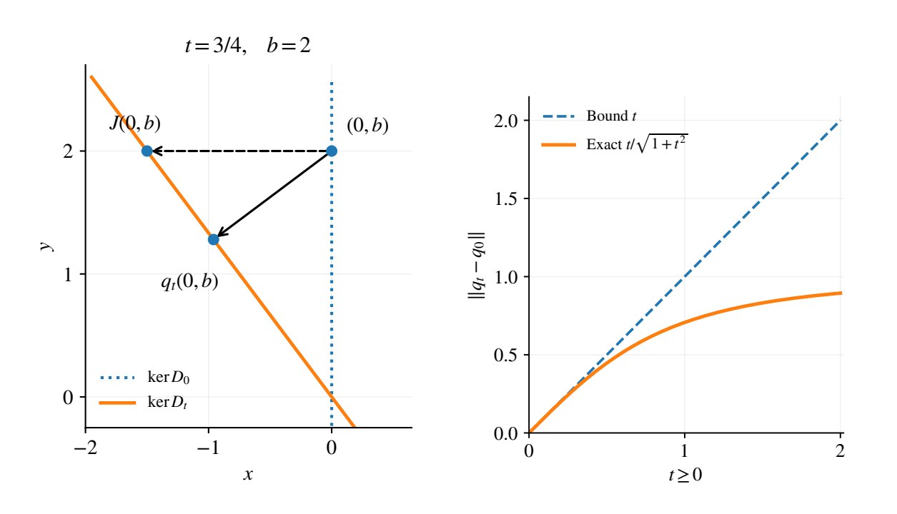
Let \(D_t(x,y)=x+ty\). Its kernel is the line \(\{(-tb,b):b\in{\mathbb R}\}\), and its orthogonal projector is
The common right inverse \(r\mapsto(r,0)\) supplies gain at most one for every \(t\), and \({\left\lVert D_s-D_t\right\rVert}=|s-t|\). The general theorem gives \({\left\lVert q_s-q_t\right\rVert}\le|s-t|\).
Proposition 21.4: Exact motion of the line
For every real \(t\),
In the small perturbation interface, kernel transport sends \((0,b)\) to \((-tb,b)\). Orthogonal projection instead sends it to \((-tb/(1+t^2),b/(1+t^2))\).
Proof
The vector \(v_t=(-t,1)\) spans \(\ker D_t\) and has squared norm \(1+t^2>0\). Projection onto this line is
which gives the matrix in (21.2). In particular it is the orthogonal projector, not merely a map whose image is contained in the kernel.
Subtract \(q_0=\operatorname{diag}(0,1)\), obtaining the symmetric matrix
The two off-diagonal entries of its square are zero, since \(-t^3+t^3=0\). Both diagonal entries are \((t^4+t^2)/(1+t^2)^2=t^2/(1+t^2)\). Thus
Pairing this identity with an arbitrary vector proves the all-vector norm formula. It bounds the operator norm above by \(|t|/\sqrt{1+t^2}\), and evaluating any unit vector gives equality. The argument includes \(t=0\), where both sides vanish.
For the common section \(A(r)=(r,0)\), the perturbation inverse leaves \(A\) unchanged because \(D_tA=I\). The constructed transport is therefore \(Jx=x-AD_tx\) on the old kernel. At \(x=(0,b)\), it gives \((-tb,b)\). Substitution into the projection formula gives instead \((-tb/(1+t^2),b/(1+t^2))\). The strict-radius theorem applies when \(|t|<1\), but these explicit line and projection calculations are valid for every real \(t\).
21.5 What fails without the hypotheses
On this page · Permalink · Source line 614
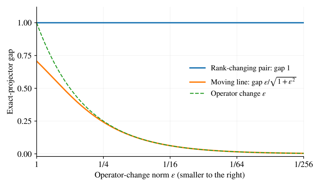
Take \(D_0=\operatorname{diag}(1,0)\) and \(D_t=\operatorname{diag}(1,t)\). The operator difference has norm \(|t|\). For every nonzero \(t\), however, the new kernel is zero, while the old kernel is the vertical axis. Their projections differ in norm by one. Operator closeness alone does not imply kernel continuity.
More generally, suppose a unit vector \(x\) is exact for the original operator but orthogonal to the new kernel. Every new residual gain \(C'\) obeys
Losing an exact direction under a small operator change forces the new gain to grow. At the strict radius boundary, \(D=I\), \(A=I\), and \(D'=0\) have \(a=\varepsilon=1\), yet \(D'\) is not surjective. Thus the strict condition in Theorem 21.2 cannot be replaced universally by a non-strict one.
21.6 Motion of the actual descent repair
On this page · Permalink · Source line 625
Compare pairs \((D,C)\) and \((D',C')\) on the same raw Hilbert space. Suppose each pair has closed local range and closed overlap range on its own locally exact subspace. Let \(G,G'\) be the resulting joint residual gains. If
then the maximum norm on the target product gives
Applying Theorem 21.1 to the joint operators, and using the actual two-stage identity of Theorem 20.1, gives
This is a comparison of the original repair maps, not a replacement definition that happens to have a similar kernel. Both the local equations and overlap conditions can change. The raw space and its inner product remain fixed.