
29 Regularization selects a protected correction
On this page · Permalink · Source line 2
A fixed budget asks how small the residual can become without exceeding an allowed correction size. Quadratic regularization reverses the emphasis. It asks for the best compromise between the residual and the size of the change. The resulting problem has a unique answer even when the exact protected equation has no solution.
That last sentence is both its usefulness and its limitation. The existence of a regularized answer is not a proof of exact realizability. The limiting behavior, rather than the mere existence of the minimizer, supplies the diagnosis.
29.1 The normal equation is derived in the protected space
On this page · Permalink · Source line 7
For \(\alpha>0\), define on \(H=\ker p\)
Both norms are the declared Hilbert norms. All minimizers below are corrections in \(H\), so preservation is exact for every parameter, not just in the limit. This is ordinary quadratic Tikhonov regularization applied to the actual protected correction operator. The standard regularization background is discussed in [6]. The proof here does not require \(T\) to be compact.
Theorem 29.1: A unique regularized correction
For every \(\alpha>0\), there is a unique minimizer
It satisfies \(T^*(r-Ta_\alpha)=\alpha a_\alpha\). For every \(a\in H\),
Proof
Step 1: the normal operator has an actual bounded inverse. Let \(B=T^*T+\alpha I:H\to H\). It is bounded and self-adjoint. For every \(h\in H\),
If \(h\ne0\), Cauchy–Schwarz and division by \({\left\lVert h\right\rVert}\) give \({\left\lVert Bh\right\rVert}\ge\alpha{\left\lVert h\right\rVert}\). The same inequality holds at zero. It implies injectivity of \(B\).
To prove closedness of its range, suppose \(Bh_n\to y\). Applying the lower bound to \(h_n-h_m\) gives
Thus \(h_n\) is Cauchy. Completeness of \(H\) supplies a limit \(h\), and continuity gives \(Bh=y\). If \(y\) is orthogonal to the range of \(B\), then for every \(h\),
Taking \(h=By\) gives \(By=0\), and injectivity gives \(y=0\). A closed subspace with zero orthogonal complement is the whole Hilbert space, so \({\operatorname{ran}} B=H\).
The inverse therefore exists. Its linearity follows from uniqueness of preimages, and its bound is \({\left\lVert B^{-1}y\right\rVert}\le\alpha^{-1}{\left\lVert y\right\rVert}\). This construction does not assume closedness of \({\operatorname{ran}} T\). It uses the positive term \(\alpha I\) in the normal operator.
Step 2: define the optimizer and prove its normal equation. Set \(a_\alpha=B^{-1}T^*r\). Then \(Ba_\alpha=T^*r\), or equivalently
Because the construction takes place in \(H=\ker p\), it already satisfies the exact protection requirement.
Step 3: prove global minimality, rather than just stationarity. Write any proposed correction as \(a=a_\alpha+h\) and set \(s=Ta_\alpha-r\). Expanding both squared norms gives
This is the asserted energy identity. It is nonnegative and, since \(\alpha>0\), vanishes only for \(h=0\). Therefore \(a_\alpha\) is the unique global minimizer. In the zero correction space, the same construction and identities reduce to its single element, zero.
A declared regularization parameter is part of the problem. A calculation that changes \(\alpha\) is solving a different optimization problem, even if the protected data and forward operator stay fixed. On the other hand, the preservation condition itself does not change with \(\alpha\).
29.2 Coordinate bases must retain the correction metric
On this page · Permalink · Source line 68
In finite dimensions, choose orthonormal coordinates in the ambient candidate and residual spaces. Let \(B\) have linearly independent columns spanning \(\ker p\). The columns of \(B\) need not be orthonormal. Write \(a=Bc\). The coefficient vector \(c\) is a representation of the correction, not necessarily an isometric one. Set
The correct coordinate equation is
The matrix \(G\) is positive definite because the columns are independent. Replacing \(G\) by the identity changes the meaning of correction size unless the chosen basis is orthonormal.
For example, let \(d(a_1,a_2)=a_1\), \(p(a_1,a_2)=a_1-a_2\), \(r=1\), and \(\alpha=1\). A basis of \(\ker p\) is the column \(B=(1,1)^{\mathsf T}\). Here \(S=1\) and \(G=2\), so the correction is \((1/3,1/3)\). Penalizing the coordinate with \(G=1\) instead gives \((1/2,1/2)\). The latter is not the optimizer for the ambient Euclidean norm. The difference is a metric change, not a discrepancy between equivalent calculations.
The executable example in this edition constructs the nullspace basis over the rationals, retains its Gram matrix, solves (29.2), and returns both the correction and an exact normal-equation residual. It also handles a zero-dimensional protected kernel without pretending that a nonzero correction exists.
29.3 Parameter monotonicity and the fixed-budget problem
On this page · Permalink · Source line 83
Proposition 29.2: Regularized answers lie on the budget frontier
If \(0<\alpha<\gamma\), then
At \(M_\alpha={\left\lVert a_\alpha\right\rVert}\),
When \(v_\alpha=r-Ta_\alpha\ne0\), its normalization is an optimizing witness in Theorem 28.2 at that budget.
Proof
Let \(A_\alpha={\left\lVert a_\alpha\right\rVert}^2\) and \(R_\alpha={\left\lVert r-Ta_\alpha\right\rVert}^2\). Comparing the two admissible minimizers in each other's objectives gives
Add these inequalities and cancel the residual terms. The result is
Since \(\gamma>\alpha\), it follows that \(A_\alpha\ge A_\gamma\). Return to the first comparison to obtain
Taking square roots, which preserves order for nonnegative numbers, proves both monotonicity statements.
At \(M_\alpha={\left\lVert a_\alpha\right\rVert}\), the vector \(a_\alpha\) is budget-feasible. If another correction \(a\) in that ball had strictly smaller residual norm, then
contradicting its defining minimality. Thus it attains the budget frontier.
For the witness statement, let \(v=r-Ta_\alpha\ne0\). The normal equation gives \(T^*v=\alpha a_\alpha\). Also \(r=v+Ta_\alpha\), hence
For \(z=v/{\left\lVert v\right\rVert}\), the support penalty is
Subtracting it from \(\langle r,z\rangle\) yields \({\left\lVert v\right\rVert}=\beta(M_\alpha)\), so this is an optimizing witness. This calculation also covers a zero correction \(a_\alpha\) with nonzero residual. If \(v=0\), normalization is unavailable, but the zero witness attains the zero budget residual.
This links a penalized calculation to a hard-budget certificate. It does not say that every larger budget must produce a different answer. Once the least-squares floor is attained, excess budget can be irrelevant. If \(T^*r=0\), every regularized correction is zero and the entire profile is constant.
29.4 The limit separates projection from actual realizability
On this page · Permalink · Source line 137
Keep \(C=\overline{{\operatorname{ran}} T}\), \(b=P_Cr\), and \(q={\left\lVert r-b\right\rVert}\). Since \(r-b\in\ker T^*\), the regularized corrections depend on \(b\), not on the component that is orthogonal to the closure of all attainable residuals.
Theorem 29.3: The regularization limit alternative
As \(\alpha\downarrow0\),
If \(b\in{\operatorname{ran}} T\), let \(a^\dagger\) be its unique minimum norm preimage. Then
If \(b\notin{\operatorname{ran}} T\), then \({\left\lVert a_\alpha\right\rVert}\to\infty\).
Proof
Step 1: identify the unavoidable component. Since \(r-b\perp\overline{{\operatorname{ran}} T}\), the adjoint identity gives \(T^*(r-b)=0\). Thus \(a_\alpha(r)=a_\alpha(b)\). For every correction the orthogonal decomposition is
In particular both the residual square and the minimum objective are at least \(q^2\).
Step 2: take the small-parameter limit in the correct order. Let \(\epsilon>0\). Since \(b\) lies in the closure of the range, choose a single \(a\in H\) with \({\left\lVert r-Ta\right\rVert}^2<q^2+\epsilon\). This \(a\) is chosen before \(\alpha\). Minimality gives
For sufficiently small \(\alpha\), the last term is below \(q^2+2\epsilon\) (and if \(a=0\) it is already below \(q^2+\epsilon\)). Hence both intervening quantities tend to \(q^2\). Their difference is \(\alpha{\left\lVert a_\alpha\right\rVert}^2\), which tends to zero. The orthogonal decomposition now implies \({\left\lVert Ta_\alpha-b\right\rVert}^2\to0\), and taking square roots gives the first two limits.
Step 3: when the projected datum is attained, obtain a uniform bound. Suppose \(b\in{\operatorname{ran}} T\). The preimage set is a nonempty closed affine subset, so projection of zero supplies its unique minimum-norm element \(a^\dagger\). Comparing with it and subtracting \(q^2\) gives
Thus \({\left\lVert a_\alpha\right\rVert}\le{\left\lVert a^\dagger\right\rVert}\) for every \(\alpha>0\). This bound does not follow merely from the previously proved vanishing weighted penalty.
Step 4: strengthen weak convergence to norm convergence. Take an arbitrary sequence \(\alpha_n\downarrow0\), or more generally positive \(\alpha_n\to0\). The bound supplies a weakly convergent subsequence \(a_{\alpha_{n_k}}\rightharpoonup a\). Since its images converge in norm to \(b\), the adjoint pairing argument of Theorem 27.2 yields \(Ta=b\). Weak lower semicontinuity gives
Minimality and uniqueness of \(a^\dagger\) force \(a=a^\dagger\). Moreover the same lower bound, together with the uniform upper bound, gives convergence of the norms to \({\left\lVert a^\dagger\right\rVert}\). In a real Hilbert space,
Thus this subsequence converges strongly. If the full positive-parameter family failed to converge strongly, there would be an \(\epsilon>0\) and parameters \(\alpha_n\to0\) whose corrections all stayed at distance at least \(\epsilon\) from \(a^\dagger\). The argument just given would produce a strongly convergent subsequence of them, a contradiction. This proves the limit for the entire parameter family.
Step 5: in the unattained case the norms tend to infinity. If \(b\notin{\operatorname{ran}} T\) and the norms failed to tend to infinity, there would exist \(M<\infty\) and positive \(\alpha_n\to0\) with \({\left\lVert a_{\alpha_n}\right\rVert}\le M\). Their images still tend to \(b\) by Step 2. Theorem 27.2 would then put \(b\) in the actual range, a contradiction. This proves divergence of the norms, not just unboundedness somewhere along the path.
The vanishing penalty \(\alpha{\left\lVert a_\alpha\right\rVert}^2\) is not a boundedness certificate for \(a_\alpha\). Its coefficient is tending to zero. In the escaping case, the penalty and residual can both tend to zero while the actual corrections diverge.
| Residual floor | Is \(b\) attained? | Limit of the protected corrections |
|---|---|---|
| \(q=0\) | Yes | Strong convergence to the nearest exact protected correction. |
| \(q=0\) | No | Residual vanishes, correction norms diverge, no exact protected answer. |
| \(q>0\) | Yes | Strong convergence to the least-squares correction of minimum norm, not an exact answer. |
| \(q>0\) | No | A positive residual floor and diverging correction norms occur together. |
The last case is not hypothetical. Let \(Tu=(u_n/n)\) on \(\ell^2\), define \(Su=(Tu,0)\) into \(\ell^2\oplus{\mathbb R}\), and take \(r=((1/n),1)\). Then \(b=((1/n),0)\) is in the closure but not the range, while \(q=1\). The same escaping corrections as before coexist with an irreducible orthogonal residual. Positive floor and unbounded correction cost are independent features.
29.5 Noise is controlled at a fixed parameter
On this page · Permalink · Source line 206
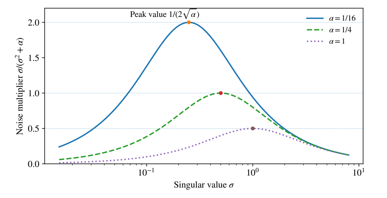
Theorem 29.4: Data sensitivity and a convergent parameter choice
For two residual data vectors \(r,\widetilde r\) with \({\left\lVert r-\widetilde r\right\rVert}\le\delta\) and the same \(T,\alpha\),
The coefficient \(1/(2\sqrt\alpha)\) is sharp over bounded linear Hilbert operators. If \(b=P_Cr\in{\operatorname{ran}} T\), \(\alpha(\delta)\to0\), and \(\delta/\sqrt{\alpha(\delta)}\to0\), then the noisy corrections converge strongly to \(a^\dagger\) as \(\delta\to0\).
Proof
Both corrections are constructed at the same positive parameter and in the same Hilbert correction space. Let \(h=a_\alpha(\widetilde r)-a_\alpha(r)\) and \(e=\widetilde r-r\). Subtract the two normal equations to obtain
Pair with \(h\) and use the adjoint identity:
Put \(t={\left\lVert Th\right\rVert}\ge0\). If \(t>0\), dropping the nonnegative penalty and dividing by \(t\) gives \(t\le\delta\). If \(t=0\), that inequality is already true. Completing the scalar square gives
Because \(\alpha>0\), taking square roots proves the correction bound. This also explains why the coefficient is \(1/(2\sqrt\alpha)\) rather than the coarser \({\left\lVert T\right\rVert}/\alpha\) obtained by bounding the inverse alone.
For sharpness at a fixed parameter, take \(H=Y={\mathbb R}\) and \(T=\sqrt\alpha\,I\). The solution map is multiplication by
Any nonzero data perturbation attains the first bound. This is worst-case sharpness across operators at that parameter, not a claim of equality for every fixed operator and every parameter.
For the limiting statement, insert the exact-data correction at the selected parameter:
The first term tends to zero by the noise/parameter hypothesis. The second tends to zero by the attained-projection case of Theorem 29.3, because the selected parameter tends to zero. Both statements require the same fixed operator and Hilbert metrics. The conclusion is a least-squares correction when the unavoidable residual component is nonzero.
The theorem does not manufacture an exact solution when \(r\) is outside the range. For the positive-floor attainable case it converges to a least-squares correction. For the unattainable projected datum it cannot produce a bounded exact-data limit. The range hypothesis must therefore precede the parameter-choice conclusion.
How to read the result
Regularization gives a unique, exactly protected answer at every positive parameter. Whether those answers converge to an exact realization, converge only to a best approximation, or escape is determined by the projected datum's actual range membership. A smooth regularized path does not erase that distinction.