
8 Banach repair and constructed split coordinates
On this page · Permalink · Source line 89
8.1 An actual complete candidate space
On this page · Permalink · Source line 90
Let \(X_n,Y_n\) be Banach spaces over a complete nontrivially normed field, with continuous linear bonding maps and uniform bounds \({\left\lVert\rho^X_n\right\rVert}\le B_X\), \({\left\lVert\rho^Y_n\right\rVert}\le B_Y\). Use the spaces of bounded operator families
The source formalization derives the required completeness from the operator spaces and their bounded product. The same differential satisfies
Thus it is a continuous linear map, and evaluation at a fixed level is continuous. These facts connect algebraic compatibility to an analytic limit argument.
8.2 From a correction operator to a projection
On this page · Permalink · Source line 102
The next statement is general. Let \(E\) be Banach, let \(d:E\to R\), \(p:E\to S\), and \(A:R\to E\) be continuous linear maps. Suppose \(pA=0\) and, for \(0\le q<1\),
The hypothesis concerns residuals of actual candidates. It need not hold for every independent vector in \(R\).
Theorem 8.1: Constructed geometric repair
Starting from \(f^{(0)}=f\), define
There is a bounded linear projection \(P_A:E\to\ker d\) with
and
It fixes every exact candidate and satisfies
Proof
Put \(r_m=df^{(m)}\). Additivity of \(d\) gives
Each \(r_m\) is the residual of an actual candidate, so the stated hypothesis applies at every iteration. Induction yields, for \(j\ge0\),
For \(n>m\), the finite triangle inequality therefore gives
Since \({\left\lVert r_m\right\rVert}\le q^m{\left\lVert df\right\rVert}\) tends to zero, this is a Cauchy estimate. Completeness of \(E\) supplies a limit, denoted \(P_Af\). Passing \(n\to\infty\) in the same norm inequality proves the required tail estimate.
Continuity of \(d\) implies \(d(P_Af)=\lim_m r_m=0\). Protection holds before taking a limit: \(pA=0\) gives \(pf^{(m+1)}=pf^{(m)}\), hence \(pf^{(m)}=pf\) for every \(m\). Continuity of \(p\) gives \(p(P_Af)=pf\). This explains why continuity of the observable belongs to this analytic statement.
For linearity, write \(L=I-Ad\), so \(f^{(m)}=L^mf\). For fixed \(f,g\) and scalars \(\lambda,\mu\),
Continuity of addition and scalar multiplication allows passage to the norm limit and proves linearity of \(P_A\). The estimate with \(m=0\) gives
so the linear map is bounded. If \(df=0\), every iterate equals \(f\), hence \(P_Af=f\). Its image is contained in \(\ker d\) and it fixes that kernel, proving surjectivity onto its stated image and \(P_A^2=P_A\). For \(q=0\) the residual vanishes after the first update and the same inequalities remain valid.
This theorem constructs the dynamics from \(A\). It does not construct a suitable \(A\) for every residual problem. That missing input can, however, be derived for a useful class of actual towers.
8.3 A right inverse from target splittings
On this page · Permalink · Source line 163
Suppose each target bonding map has a continuous linear section
Assume the propagation gap
For \(r\in R\), recursively set
Theorem 8.2: Split tower correction
The recurrence defines a continuous linear map \(A:R\to E\) with
The operator \(P=I-A\partial\) is an exact projection and
Proof
Let \(\theta=SB_X<1\). The number \(K=S/(1-\theta)\) is nonnegative and satisfies
Fix \(r\in R\) and define its coordinates recursively as in (8.3). The initial coordinate has norm zero. If \({\left\lVert(Ar)_n\right\rVert}\le K{\left\lVert r\right\rVert}_\infty\), submultiplicativity of operator norms gives
Induction proves the estimate at every coordinate, so the recursively defined family actually belongs to the bounded product \(E\).
The coordinate recurrence preserves addition and scalar multiplication, starting from the zero initial coordinate. Induction therefore proves these laws for the family map \(A\). Its uniform estimate proves \({\left\lVert A\right\rVert}\le K\), giving a continuous linear map with the claimed domain and codomain.
For every \(n\), apply the target restriction to the recurrence. The equation \(\rho^Y_ns_n=I\) gives
Coordinate equality yields the operator identity \(\partial A=I_R\). In particular this identity holds for every bounded residual, not just residuals already known to lie in the image.
Set \(P=I-A\partial\). Then
The expression \(2A\partial\) abbreviates addition of the same operator twice and uses no division by two. Every exact \(f\) is fixed because \(\partial f=0\). Since \((Ar)_0=0\), the seed of \(Pf\) is \(f_0\). Finally \(f-Pf=A\partial f\), and the bound on \(A\) gives the asserted residual estimate. The denominators above are justified exactly by the strict propagation gap.
The surjectivity is onto all bounded residual families. It is stronger than the assertion that some exact output can be assigned to each candidate. The gap and the chosen splittings are genuine inputs.
8.4 Protected information beyond the seed
On this page · Permalink · Source line 223
When the target grows, its new kernel directions are independent information. Define
Each \(N_n(f)\) lands in \(\ker\rho^Y_n\). The observable \(p_L\) retains both the seed and every new output component, relative to the chosen sections.
Theorem 8.3: Split coordinate theorem
The observable is a bounded projection with \(p_LA=0\) and \(p_LP=p_L\). It separates exact candidates. If
then
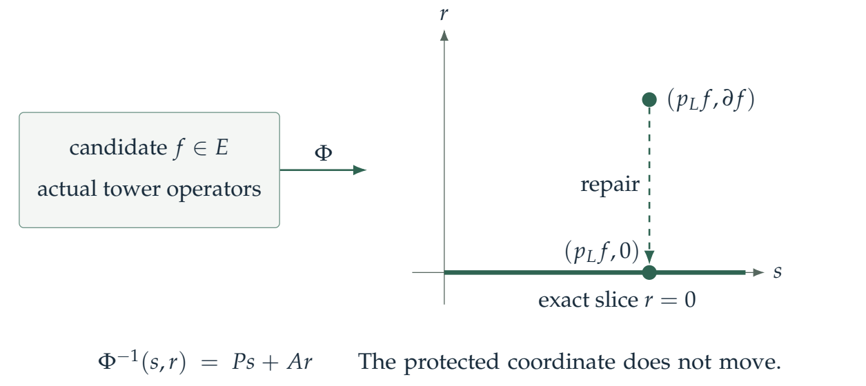
Repair becomes \((s,r)\mapsto(s,0)\). It is the unique exact repair preserving \(p_Lf\).
Proof
Put \(B_n=I-s_n\rho^Y_n\). Since \(\rho^Y_ns_n=I\), direct multiplication gives
Moreover, \(B_ny=y\) whenever \(\rho^Y_ny=0\). Thus \(B_n\) really projects onto the target kernel. Its norm is at most \(1+SB_Y\). Coordinate zero of \(p_L\) is the identity, and every later coordinate applies \(B_n\), so \(p_L^2=p_L\) and \({\left\lVert p_L\right\rVert}\le1+SB_Y\). In particular the formula defines a map on the bounded product, not just on arbitrary coordinate families.
The recurrence for \(Ar\) gives zero seed and places \((Ar)_{n+1}\) in the image of \(s_n\). The identities just proved make all its innovations zero. Therefore \(p_LA=0\), and
We next prove separation on the exact space. If \(f\) is exact, its restriction equation rewrites as
Two exact families with the same seed and innovations agree first at level zero and then at every later level by this recurrence. More generally, if two arbitrary families have the same observable and differential, their difference is exact with zero observable, so separation on the exact space makes their difference zero.
The proposed chart has the claimed target because \(p_L(p_Lf)=p_Lf\). Given \(s\in\mathcal S_L\) and \(r\in R\), set \(f=Ps+Ar\). The preceding identities and \(\partial A=I\) give
This proves one round trip. For the other, \(f\) and \(P(p_Lf)+A\partial f\) have the same observable and residual, so the joint separation just proved identifies them. All maps are linear and bounded on their indicated subspaces and finite products, establishing a continuous linear equivalence.
Finally, \(Pf\) has coordinates \((p_Lf,0)\). Any exact answer with the same observable has those same two coordinates, hence equals \(Pf\). This uniqueness is relative to the complete observable of seed and innovations. It is not obtained by assuming that the seed alone determines an exact growing-target family.
This is an actual analytic coordinate equivalence, not generally an isometry. The protected coordinate depends on the declared splitting. It should not be called an intrinsic semantic coordinate without a further comparison theorem.
8.5 A growing example and the gap boundary
On this page · Permalink · Source line 275
Use \(X_n=Y_n={\mathbb R}^{n+1}\) with maximum norms. Let \(\pi_n\) delete the last coordinate, take \(\rho^X_n=\tfrac12\pi_n\), \(\rho^Y_n=\pi_n\), and let \(s_n\) append zero. Then \(S=B_Y=1\), \(B_X=1/2\), and \(K=2\).
Example 8.4: Repair of the identity family
The bounded candidate \(f_n=I\) is not exact. Its repair is
The new last output row is retained at every stage while inherited rows are propagated by the factor \(1/2\).
Proof
At level zero the value is one. Exactness forces every inherited row at the next level to be one half of its previous value. Preservation of the innovation forces the new row to remain the corresponding identity row. Induction gives the displayed diagonal.
For constant real scalar identity towers, by contrast, \((\partial f)_n=f_{n+1}-f_n\). The constant residual \(r_n=1\) has no bounded primitive, since any primitive satisfies \(f_n=f_0+n\). Here \(SB_X=1\). This counterexample excludes discarding the gap indiscriminately. It does not prove that the gap is necessary for every individual tower. Exact repair preserving the initial coordinate still exists in this constant example, by replacing a candidate with its initial constant family. Surjectivity onto all bounded residuals does not follow from that repair.
8.6 What is canonical
On this page · Permalink · Source line 292
For fixed splitting and protected observable, the repair above is unique. Changing the splitting can change both the observable and the repaired answer. In the growing example, replace \(s_n(y)=(y,0)\) by \(s_n'(y)=(y,y_0)\). At the first positive level, repair of the identity becomes
Both are exact continuations for their respective innovation profiles and have the same seed. Thus a unique answer for a declared preservation problem is not an answer independent of all preservation choices.