
32 Coordinates, noise, and a justified stopping rule
On this page · Permalink · Source line 1
A certificate can be exact and still be interpreted incorrectly. Two common errors are to measure a coordinate covector with the wrong norm, or to keep a solver tolerance fixed while sending the regularization parameter to zero. Both change what a small reported number means.
32.1 The residual of the coordinate equation is a covector
On this page · Permalink · Source line 4
In finite dimensions, use orthonormal coordinates in the ambient candidate and residual spaces. Let the columns of \(B\) form an arbitrary basis of \(H=\ker p\), not necessarily an orthonormal one. Write \(a=Bc\), \(S=dB\), and \(G=B^{\mathsf T}B\). As before, \(G\) is positive definite. For an inexact coefficient vector \(c\), the residual of the coordinate normal equation is
The vector \(q\) stores pairings against basis vectors. It is not the coordinate vector of the Hilbert normal residual unless the basis is orthonormal.
Proposition 32.1: The invariant norm of a coordinate certificate
The actual normal residual is
For any invertible change of basis \(B'=BC\), the same proposed correction has
and
Proof
Because \(B\) has independent columns, for every nonzero coefficient vector \(c\),
Thus \(G\) is positive definite and invertible. The matrix \(P=BG^{-1}B^{\mathsf T}\) is symmetric and obeys
Its range is precisely the column space \(H\), so it is the orthogonal projection onto the entire permitted correction space.
The restricted Hilbert normal residual is
Substitute \(S=dB\), \(G=B^{\mathsf T}B\) and the expression for \(P\):
Equivalently \(q=B^{\mathsf T}g\) records the pairings of \(g\) with the basis columns. Its squared Hilbert norm is
using symmetry of \(G^{-1}\). This proves both coordinate formulas.
For the basis change \(B'=BC\), the same ambient vector is represented by \(c'=C^{-1}c\). Also \(S'=SC\) and \(G'=C^{\mathsf T}GC\). Substitute these formulas into the new coordinate normal equation:
The inverse metric is \((G')^{-1}=C^{-1}G^{-1}(C^{\mathsf T})^{-1}\). Hence
For a zero-dimensional kernel these are empty matrices and zero vectors, and the resulting scalar norm is zero. The spanning assumption is indispensable: a basis of a proper subspace would compute a projection to a different correction problem.
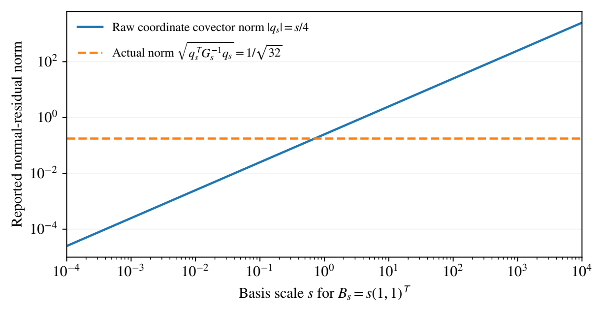
In the previous example, \(B=(1,1)^{\mathsf T}\), \(G=2\), and the proposal \(c=1/4\) gives \(q=-1/4\). Thus \(q^{\mathsf T}G^{-1}q=1/32\), as required. Replacing \(B\) by \(sB\) changes \(q\) to \(sq\) and \(G\) to \(s^2G\). The Euclidean norm of the coordinate covector can be made arbitrarily small or large by changing the nonzero scalar \(s\). The actual correction, normal residual, and certified error do not change.
The finite verifier checks that a supplied basis spans the whole protected kernel. A basis of a smaller subspace might give a correct certificate for that smaller optimization problem while missing an allowed direction that decreases the objective. The rank, kernel-membership, and independence checks therefore belong to the certificate contract.
32.2 Separate data error, numerical error, and regularization bias
On this page · Permalink · Source line 77
Let \(r\) be the intended datum and \(\widetilde r\) the measured datum. Suppose
The maps \(T,p\) and their Hilbert metrics remain fixed. By Theorem 31.1 and the fixed-parameter part of Theorem 29.4,
The first term is the solver's contribution. The second is the worst-case propagation of data error. They should not be collapsed into one unqualified residual tolerance.
Theorem 32.2: A consistent inexact stopping rule
Assume the projected intended datum belongs to the actual range of \(T\), with minimum-norm preimage \(a^\dagger\). Along a sequence of positive parameters and measured problems, suppose
If the proposed corrections \(a_n\in H\) satisfy the displayed data and normal-residual bounds, then \(a_n\to a^\dagger\) in norm. At every index,
Proof
At index \(n\), distinguish two exact minimizers: let \(\widetilde a_n=a_{\alpha_n}(\widetilde r_n)\) solve the measured problem and let \(a_n^0=a_{\alpha_n}(r)\) solve the intended-data problem. All three corrections, including the proposal \(a_n\), belong to the same space \(H\).
The supplied normal-residual bound is for the measured datum. Therefore Theorem 31.1 applies first to that problem and gives
The pointwise data estimate in Theorem 29.4, at the same parameter, then gives
Insert these two intermediate vectors between \(a_n\) and \(a^\dagger\) in the triangle inequality to obtain the displayed three-term estimate.
The first term tends to zero by the solver-tolerance hypothesis and the second by the data/parameter hypothesis. Since the projected intended datum is attained and \(\alpha_n\to0\), the last term tends to zero by Theorem 29.3. For a direct epsilon argument, make each term smaller than one third of a prescribed tolerance beyond its own threshold and take the maximum of the three thresholds. This gives norm convergence of the proposals.
Protection is not merely asymptotic: \(a_n\in\ker p\) implies \(p(f-a_n)=pf\) at every index. The proof compares no changing operators or changing kernels. Both the pointwise certificate and the convergence conclusion have formal counterparts under these hypotheses.
The accompanying Lean formalization includes the pointwise estimate (32.2), the regularization limit, and the resulting convergence theorem. Their statements retain the same fixed operator, Hilbert geometry, and attainment requirements.
32.3 Retaining the explicit diagonal rate with an inexact solver
On this page · Permalink · Source line 126
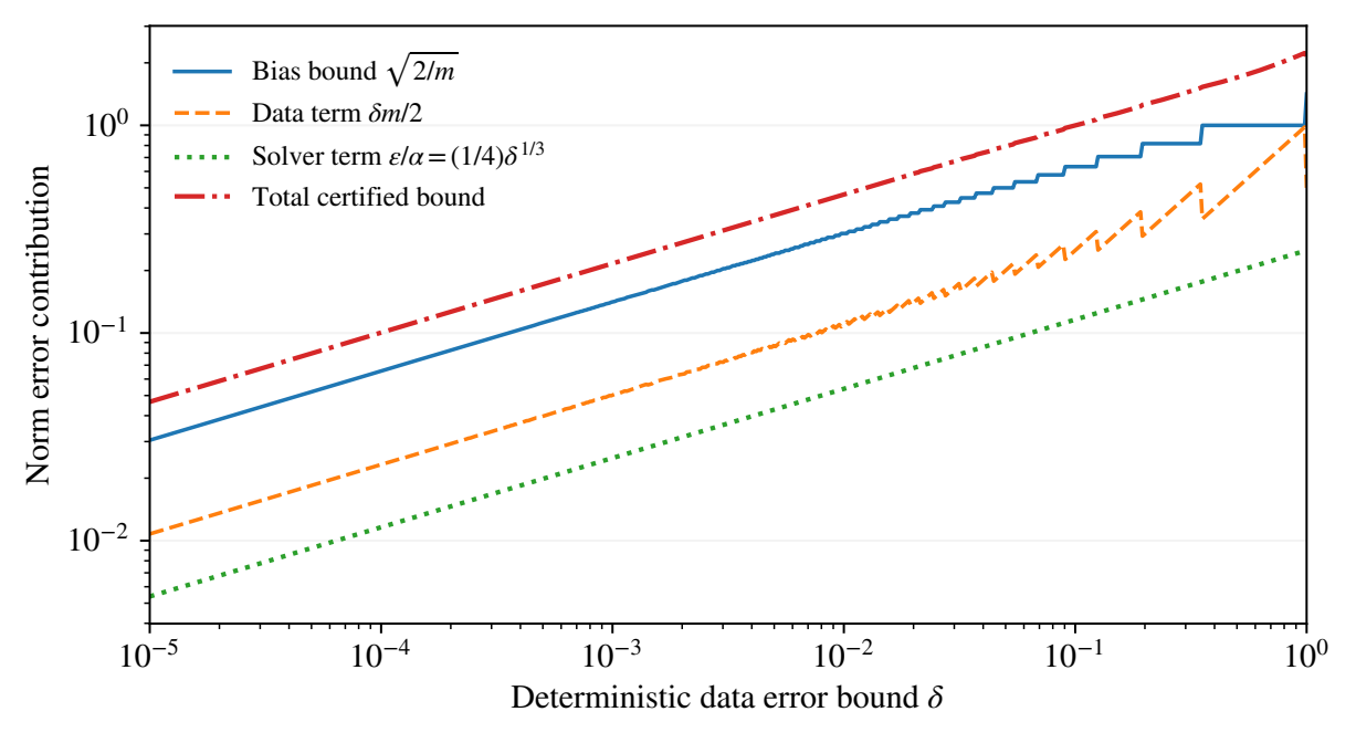
For the attainable datum of Corollary 30.3 and \(0<\delta\le1\), take \(m=\lceil\delta^{-2/3}\rceil\) and \(\alpha=m^{-2}\) as before. If an inexact solver satisfies
then the same argument gives
Thus the inner solve can retain the proven outer accuracy if its normal residual decreases on the scale \(\alpha\delta^{1/3}\). Since \(\alpha\) is on the scale \(\delta^{4/3}\), the corresponding normal-residual scale is \(\delta^{5/3}\), with the stated ceiling factors retained in the exact rule. This is a sufficient rule for this problem, not a universal optimal stopping law.
The declaration DiagonalRegularization.diagonal_inexact_rounded_rate formalizes this specialization for the actual infinite diagonal operator. Its hypotheses bound both the data error and the normal residual evaluated against the measured datum. It retains the literal ceiling in \(m\) and derives the exact-data bias estimate within the model.
For the escaping datum, the same rule does not create convergence to a nonexistent protected Hilbert answer. It only makes the numerical proposals track the regularized path accurately. Tracking an escaping path and converging to a realization are different conclusions.
32.4 The executable verification contract
On this page · Permalink · Source line 144
The program takes \(d,p,f,\alpha\) and a proposed ambient correction, with optional measured residuals, a full kernel basis, and an independent dual witness. It rejects a correction that changes the protected data and checks the basis's dimensions, rank, and kernel membership. It does not silently project a rejected proposal into another problem.
The output records \(f-a\), protection before and after, measured fit, actual model residual, the Gram-corrected normal certificate, objective values, and squared error bounds. Verification recomputes the record without calling an optimizer. Independent determinant-based tests compare the bounds with actual errors in small ambient constrained systems. A certificate establishes consistency with its included problem, not authentication that this is the externally intended task.
How to read the result
A certificate needs a declared target. Fit measures agreement with data. The normal residual bounds optimizer error at a specified parameter. The duality gap bounds objective error. A realization theorem is still needed to conclude convergence to an intended exact object.