
30 A complete regularization diagnostic for the escaping model
On this page · Permalink · Source line 1
The abstract alternatives become explicit for the diagonal model. They also answer a natural objection to the hard prefix corrections: perhaps a smoother correction could fit increasingly well without escaping. It can fit more efficiently, but it cannot avoid the obstruction.
30.1 The entire regularized family is explicit
On this page · Permalink · Source line 4
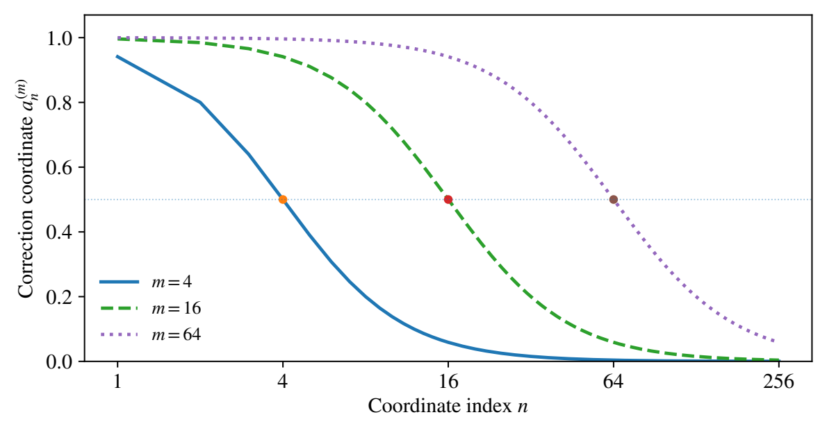
Use \(Tu=(u_n/n)\) and \(r=w=(1/n)\) as in Section 26. Choose \(\alpha=m^{-2}\) for an integer \(m\ge1\). The normal equation in each coordinate gives
The repaired ambient candidate is \((-a^{(m)},1)\). Its protected coordinate is one for every \(m\).
Proposition 30.1: Energy, residual, and certified tails
The displayed \(a^{(m)}\) belongs to \(\ell^2\) and is the unique regularized correction at \(\alpha=m^{-2}\). Set
Then
For the sums \(A_{m,K},B_{m,K}\) through any integer \(K\ge m\),
Proof
For \(n>m\), one has \((a_n^{(m)})^2\le m^4/n^4\), so the correction sequence is square-summable. The diagonal operator is bounded with norm one, and \(w=(1/n)\in\ell^2\), hence the residual sequence is also in \(\ell^2\). The operator is self-adjoint, and the coordinate equality
proves \(T^*v^{(m)}=\alpha a^{(m)}\) as an equality of Hilbert vectors. Theorem 29.1 therefore identifies this actual infinite vector as the unique minimizer, rather than just a coordinatewise candidate.
For \(1\le n\le m\), \(m^2/(m^2+n^2)\ge1/2\). There are \(m\) such coordinates, so \(A_m\ge m/4\). For the upper bound, the first \(m\) squares are at most one, and the decreasing function \(x^{-4}\) gives
Thus \(A_m\le m+m^4/(3m^3)=4m/3\).
For \(n\le m\), the residual square is at most \(n^2/m^4\). The sum-of-squares estimate
holds for \(m\ge1\), so this part contributes at most \(1/m\). For \(n>m\), each residual square is at most \(1/n^2\), whose tail is at most \(1/m\). This proves \(B_m\le2/m\).
For the lower bound, \(n>m\) implies \(m^2+n^2\le2n^2\), hence
The other direction of the decreasing-function integral comparison gives
This proves \(B_m\ge1/(4(m+1))\).
Finally, for \(K\ge m\), both omitted tails consist of nonnegative terms. Bound the first by \(m^4\sum_{n>K}n^{-4}\) and the second by \(\sum_{n>K}n^{-2}\). The same upper integral comparisons give the two certified remainders in (30.2). No finite truncation is substituted for an equality of infinite energies.
Thus the correction norm grows on the order of \(\sqrt m\), the residual norm decays on the order of \(m^{-1/2}\), and the penalty \(\alpha A_m=A_m/m^2\) tends to zero. The smooth correction avoids the hard discontinuity at a prefix boundary, but it still approaches the forbidden constant sequence coordinate by coordinate.
30.2 The sharp asymptotic correction cost
On this page · Permalink · Source line 67
The preceding bounds establish divergence and decay. The leading constant can also be computed, which permits a meaningful comparison with hard prefix repair.
Theorem 30.2: A sharp budget asymptotic for the diagonal datum
As \(m\to\infty\),
For the exact budget profile of this infinite problem,
The hard prefix correction at budget \(M=\sqrt N\) instead has
Proof
Step 1: control the infinite Riemann sums uniformly. Define
Then \(A_m/m=m^{-1}\sum_{n\ge1}f(n/m)\) and \(mB_m=m^{-1}\sum_{n\ge1}g(n/m)\). Fix \(L\ge2\) and put \(N=\lfloor mL\rfloor\). On \([0,L]\), both functions are uniformly continuous. If \(\omega_f(h)\) is a modulus of continuity there, comparison on the \(N\) intervals of length \(1/m\) gives
The missing interval \([N/m,L]\) has length below \(1/m\) and a bounded integrand, so it contributes a term tending to zero. The same argument applies to \(g\). This proves convergence of each truncated sum to its integral on \([0,L]\).
The tails require a bound independent of sufficiently fine discretization. Since \(N\ge mL/2\), the inequalities \(f(x)\le x^{-4}\) and \(g(x)\le x^{-2}\) give
The integral tails are at most \(1/(3L^3)\) and \(1/L\). Given an error tolerance, choose \(L\) first to control both discrete and integral tails, then choose \(m\) to control the compact-interval sums. This justifies passing from finite-interval Riemann convergence to the full half-line sums. No uncontrolled interchange of two infinite limits is involved.
Step 2: evaluate the integrals. The substitution \(x=\tan\theta\) gives \(dx=\sec^2\theta\,d\theta\) and \(1+x^2=\sec^2\theta\), so
Step 1 now proves the two stated asymptotics.
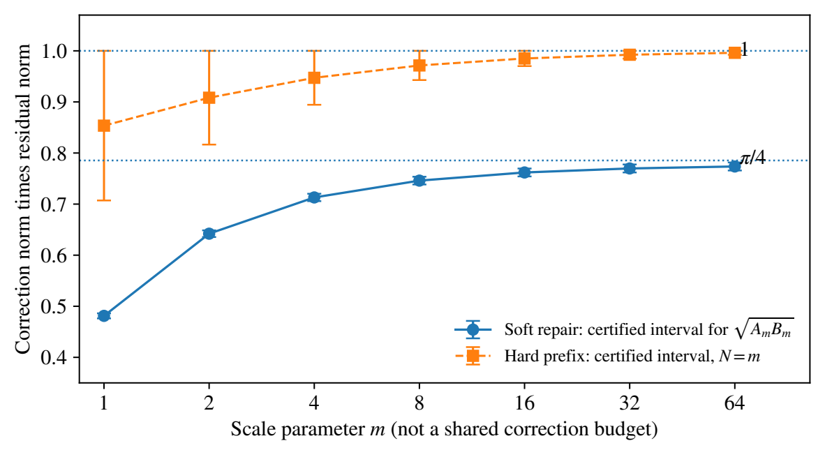
Step 3: move from regularization parameters to arbitrary budgets. Set \(M_m=\sqrt{A_m}\). Every positive coordinate \(m^2/(m^2+n^2)\) increases strictly with \(m\), so \(A_m\), and hence \(M_m\), increases strictly. Since \(A_m/m\to c=\pi/4>0\), these budgets tend to infinity and
Proposition 29.2 identifies \(\beta(M_m)=\sqrt{B_m}\). Thus
For every sufficiently large \(M\), choose \(m\) with \(M_m\le M\le M_{m+1}\). Monotonicity of \(\beta\) gives
The lower bound is \((M_m/M_{m+1})[M_{m+1}\beta(M_{m+1})]\) and the upper is \((M_{m+1}/M_m)[M_m\beta(M_m)]\). Both tend to \(c\), proving the full budget limit, not merely convergence on a selected subsequence of budgets.
Step 4: compare the hard-prefix method. That correction has norm \(\sqrt N\) and residual square \(\sum_{n>N}n^{-2}\). Integral comparison yields
Taking the limit and then a square root gives its leading product one. The two constants are consequently compared at large actual correction budgets, rather than at arbitrarily equated parameter labels.
At large matched correction budgets, the optimal soft repair therefore has about \(\pi/4\) times the hard-prefix residual. This improves the efficiency of approximation, not the existence result. Both residuals tend to zero only as the budget tends to infinity. The limiting constant is a calculation for this declared model, not a universal regularization efficiency factor.
30.3 The same operator has an attainable datum
On this page · Permalink · Source line 145
Change only the residual to \(b_n=1/n^2\). Its minimum norm preimage is \(a^\dagger_n=1/n\in\ell^2\). At \(\alpha=m^{-2}\), the regularized correction is
The bias square is exactly the previously computed \(B_m\). This links the two cases without conflating their existence hypotheses: the escaping residual of one problem is the regularization bias of an attainable problem.
Corollary 30.3: An explicit noisy attainable repair
For the attainable datum \(b=(1/n^2)\), suppose \({\left\lVert\widetilde b-b\right\rVert}\le\delta\) with \(0<\delta\le1\). Choose
Then the noisy regularized correction satisfies
Proof
The exact-data bias has coordinates \(n/(m^2+n^2)\), so its squared norm is precisely \(B_m\). By Proposition 30.1,
Theorem 29.4 at the same parameter gives
The triangle inequality proves the first bound.
Because \(0<\delta\le1\), the number \(u=\delta^{-2/3}\) is at least one. The ceiling satisfies \(u\le m<u+1\le2u\). Therefore
Adding these estimates proves the displayed rate with every ceiling factor accounted for. The positive-noise condition is needed to define this particular finite integer choice. The statement does not prescribe an infinite \(m\) at \(\delta=0\), nor does it use a probabilistic assumption on the perturbation.
This is a deterministic guarantee for the specified datum and Hilbert noise bound. It is not a statistical confidence statement. The identical parameter rule in the escaping problem cannot produce convergence to an exact protected Hilbert solution, because no such solution exists.
30.4 What the calculation permits a machine to certify
On this page · Permalink · Source line 188
The finite program can check a normal equation, exact preservation, and a quadratic optimality identity. It can return a dual witness ruling out a smaller residual at a given budget. In the infinite diagonal example it can return partial sums together with rational tail enclosures. Those are distinct certificates with distinct conclusions.
None of them alone establishes unrestricted semantic realizability. The bounded-budget theorem needs a genuinely uniform bound. The exactification theorem needs control of candidate movement. The regularization limit needs actual attainment of the projected datum. The repeated appearance of a small residual does not replace any of those hypotheses.
The useful next diagnostic is therefore not just “Did the residual decrease?” It is “What happened to the correction norm, what quantity was preserved, and what existence theorem applies to this datum?”