
22 Reading a stability certificate
On this page · Permalink · Source line 1
A numerical residual becomes useful only after it is tied to an operator, a norm, and a conclusion. This section separates uncertainty in a measured residual from uncertainty in the operator itself. It also distinguishes closeness to a reference exact space from closeness to a changed one. All estimates below refer to the actual canonical Hilbert projection used earlier.
22.1 The statement carried by a certificate
On this page · Permalink · Source line 4
Let \(D:E\to R\) be bounded linear from a real Hilbert space into a real normed space. A residual certificate with gain \(C\ge0\) is the universally quantified estimate
A reported number \(C\) is not a certificate unless this estimate has been justified in the stated model. A successful test at one input is likewise not the universally quantified estimate.
Suppose the measured vector is \(y\), with a certified error radius \(\eta\) such that \({\left\lVert Dx-y\right\rVert}\le\eta\). The triangle inequality converts the measured ball into a bound for the true residual.
Proposition 22.1: Measurement and operator uncertainty
With the reference certificate above,
More generally, let \(\widetilde D:E\to R\) be the bounded linear operator actually used in the measurement. If
then
The projection in this conclusion is still the projection for the reference operator \(D\).
Proof
The first assertion follows from \({\left\lVert Dx\right\rVert}\le{\left\lVert y\right\rVert}+\eta\). For the second, decompose
Its norm is at most \(\varepsilon{\left\lVert x\right\rVert}+\eta+{\left\lVert y\right\rVert}\). Apply the reference residual certificate.
The input-size term has a mathematical purpose. A small error in an operator can produce a large error on a large input. It cannot generally be replaced by a number depending only on the measured residual. Even a measurement of zero may reflect a difference between the measured kernel and the reference kernel.
22.2 A vanishing measured residual can still miss the reference space
On this page · Permalink · Source line 41
For a concrete family, take \(E={\mathbb R}^2\) with the Euclidean norm and \(R={\mathbb R}\), and define
The reference projection is \(q(a,b)=(0,b)\), its least residual gain is one, and \({\left\lVert D-\widetilde D\right\rVert}\le|t|\). On the input \(x=(-tB,B)\), the measured operator returns exactly zero. Its distance to the reference kernel is nevertheless \(|tB|\).
Setting \(\eta=0\) and \(y=0\) in (22.1) gives the valid upper bound \(|t|\sqrt{1+t^2}|B|\). Deleting the input-size term would give zero and would be false whenever \(tB\ne0\). The input is exact for the changed model and not exact for the reference model. This is precisely the distinction that the estimate is designed to retain.
There is no statistical assertion here. The error radii are mathematical inputs. Estimating them from noisy observations, unknown dynamics, or a fitted model is an additional task that requires its own assumptions and evidence.
22.3 A preserved kernel gives a stronger conclusion
On this page · Permalink · Source line 52
A useful regime occurs when the changed operator annihilates every old exact vector:
This says that the old kernel is contained in the new kernel. Equality is not assumed. Let \({\left\lVert D-\widetilde D\right\rVert}\le\varepsilon\) and suppose the strict budget \(C\varepsilon<1\) holds.
Theorem 22.2: Kernel preservation and a strict error budget
Under these hypotheses,
For a measurement with \({\left\lVert\widetilde D x-y\right\rVert}\le\eta\), the bound becomes
Thus the exact space is unchanged and the residual gain degrades by an explicit factor.
Proof
Let \(q=P_{\ker D}\), and write \(u=x-qx\). The stated kernel inclusion makes both \(Dqx\) and \(\widetilde Dqx\) zero. Hence \(Du=Dx\) and \(\widetilde Du=\widetilde Dx\). Applying the reference residual bound to \(u\), whose projection onto \(\ker D\) is zero, gives
Subtract the final term. The strict inequality \(C\varepsilon<1\) makes \(1-C\varepsilon\) positive, so division preserves the inequality and gives the claimed residual estimate. This also covers \(C=0\) without division by \(C\).
If \(\widetilde Dx=0\), the same estimate forces \(u=0\), hence \(x=qx\in\ker D\). This is the inclusion not initially assumed. Combining it with the supplied inclusion proves \(\ker\widetilde D=\ker D\), and their orthogonal projections coincide in the fixed Hilbert geometry. Finally \({\left\lVert\widetilde Dx-y\right\rVert}\le\eta\) gives \({\left\lVert\widetilde Dx\right\rVert}\le{\left\lVert y\right\rVert}+\eta\). Substitution proves the measured certificate. The kernel-preservation hypothesis is what removed \(qx\) before applying the perturbation estimate. Without it, one obtains a term proportional to \({\left\lVert x\right\rVert}\), not the absorbable term proportional to \({\left\lVert u\right\rVert}\).
This result does not require the reference operator to be surjective. It is different from the split-surjective perturbation theorem, which allows the kernel to move and constructs an actual transport between the old and new kernels. Both theorems have a strict quantitative radius, but they retain different structural data.
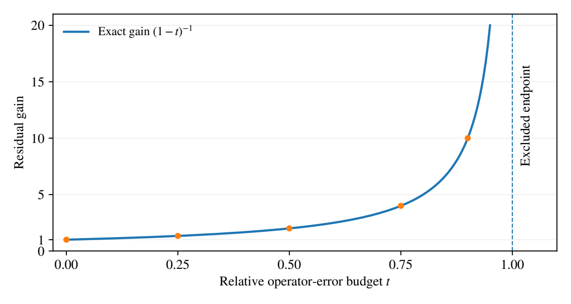
For \(D(a,b)=a\) and \(\widetilde D(a,b)=(1-t)a\), with \(0\le t<1\), the kernel is preserved and the exact gain is \(1/(1-t)\). The bound is attained on transverse inputs. At \(t=1\), the changed operator is zero and its kernel becomes all of \({\mathbb R}^2\). This illustrates why the strict endpoint cannot simply be included.
22.4 Select the theorem by its conclusion
On this page · Permalink · Source line 92
The following distinctions organize the estimates without turning them into competing formulas.
| Available information | Structural hypothesis | Certified conclusion |
|---|---|---|
| Reference gain and measured error | None on a changed kernel | Distance to the reference kernel, with an input-size term |
| Reference gain and small operator change | Old kernel preserved | Same kernel and a degraded gain |
| Two residual gains | Same source Hilbert geometry | Distance between the two orthogonal projectors |
| A right inverse and a strict radius | Split surjectivity | A new right inverse and an equivalence of moving kernels |
A claim about the new exact space cannot be obtained by silently replacing the reference projector in the first row. Conversely, a theorem that establishes equality of kernels under preservation need not be weakened to a moving-kernel estimate when the stronger hypothesis is actually available.
22.5 Norm conventions are part of the certificate
On this page · Permalink · Source line 108
On a finite family of real Hilbert fibers, the maximum norm and the Euclidean product norm satisfy
where \(n\) is the number of components. The first inequality follows because each squared component is one term in the sum. The second follows by bounding every component by the maximum. These inequalities transfer bounds with explicit dimension factors. They do not assert that the same numerical best constant remains optimal.
The graph chapters use the maximum norm on vertex and directed-edge products unless a different geometry is declared. The nearest-point statements use a Hilbert source norm. In the worked graph calculations that follow, selecting one orientation and using a sum of squared residuals defines a different numerical operator model. It has the same edge-exactness equations for an isometric connection, but a different residual norm.
A repair certificate should therefore identify its candidate space, residual map, preserved data, norms, gain, and error budgets. The exact equation alone does not specify these quantities. Explicitly retaining them is what makes a numerical conclusion transportable between examples.