Paper VIII: Discovery and exact packet compilation

9 Discovery and exact packet compilation

On this page · Visual guide: The objects and their contracts · Permalink · Source line 1459

9.1 Exact spectral discovery

On this page · Permalink · Source line 1461

Standard fact 9.1: Simultaneous spectral decomposition

A finite family of pairwise commuting normal matrices admits a common orthonormal basis of joint eigenvectors. The joint eigenspaces associated with distinct eigenvalue tuples give the coarsest orthogonal packet system on which every matrix in the family acts as a scalar.

Permalink · Source line 1463 · Claim record · Lean coverage · Code · Worked examples

Proposition 9.2: Exact block discovery certificate

For an orthogonal packet system \((P_\alpha)\), define the block diagonal compression

\[ \Pi_{{\mathcal P}}(A) = \sum_\alpha P_\alpha AP_\alpha. \]

Then

\[ \boxed{ {\left\lVert A-\Pi_{{\mathcal P}}(A)\right\rVert}_{\rm F}^2 = \sum_{\alpha\neq\beta} {\left\lVert P_\beta AP_\alpha\right\rVert}_{\rm F}^2. } \]

In operator norm,

\[ \boxed{ {\left\lVert A-\Pi_{{\mathcal P}}(A)\right\rVert}_2 \leq \sum_{\alpha\neq\beta} {\left\lVert P_\beta AP_\alpha\right\rVert}_2. } \]

Thus any proposed packet discovery has an exact finite residual certificate after its projectors are known.

Read proof · Visual guide: Twelve small blocks, one coherent error · Read statement and proof side by side · Permalink · Source line 1467 · Claim record · Lean coverage · Code · Worked examples

Proof of Proposition 9.2

Distinct matrix blocks are orthogonal in the Hilbert Schmidt inner product. Their squared Frobenius norms therefore add. The operator norm estimate follows from the triangle inequality.

Back to statement · Read statement and proof side by side · Permalink · Source line 1495 · Claim record · Lean coverage · Code · Worked examples

This supplies one exact discovery regime and one exact a posteriori certificate. Perturbation of spectral packets requires a gap. The Davis Kahan theorem gives quantitative control for Hermitian spectral subspaces under such a gap [DavisKahan1970]. Randomized low rank discovery supplies another controlled regime [HalkoMartinssonTropp2011], [MartinssonTropp2020]. Neither result gives globally optimal packet discovery for arbitrary operators.

Permalink · Source line 1499

9.2 Candidate packet trees

On this page · Permalink · Source line 1501

Definition 9.3: Candidate representation tree

A candidate representation tree is a finite rooted tree. Every node \(v\) has

\[ \kappa_v\geq0, \qquad \epsilon_v\geq0, \]

representing the cost and error of keeping \(v\) as one leaf. Every internal node also has a split overhead \(\sigma_v\geq0\). An admissible pruning contains exactly one selected node on every root to terminal path.

Permalink · Source line 1503 · Claim record · Lean coverage · Code · Worked examples

The cost and error of a pruning \({\mathcal L}\) are

\[ {\operatorname{cost}}({\mathcal L}) = \sum_{v\in{\mathcal L}}\kappa_v + \sum_{u\text{ split}}\sigma_u \]

and

\[ {\operatorname{err}}({\mathcal L})=\sum_{v\in{\mathcal L}}\epsilon_v. \]

The model can include arithmetic, storage, launch, transfer, and precision costs inside \(\kappa_v\). It remains exact only when the declared totals are additive.

Permalink · Source line 1513

Theorem 9.4: Exact Lagrangian packet compiler

Fix \(\lambda\geq0\) and define

\[ J_\lambda({\mathcal L}) = {\operatorname{cost}}({\mathcal L}) + \lambda{\operatorname{err}}({\mathcal L}). \]

For every node \(v\), set

\[ K_\lambda(v) = \kappa_v+\lambda\epsilon_v \]

and

\[ S_\lambda(v) = \sigma_v + \sum_{w\in\operatorname{child}(v)}F_\lambda(w). \]

For a terminal node, set

\[ F_\lambda(v)=K_\lambda(v). \]

For an internal node, the recurrence

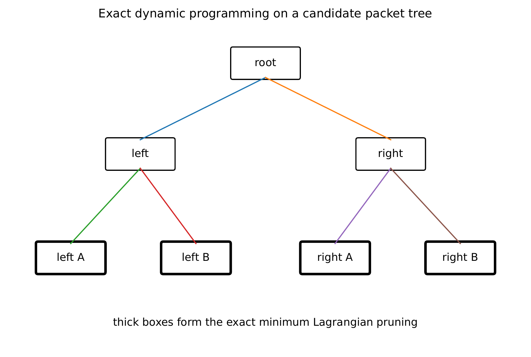
\[ \boxed{ F_\lambda(v) = \min\{K_\lambda(v),S_\lambda(v)\} } \]

computes the exact minimum Lagrangian objective over every admissible pruning of the subtree rooted at \(v\).

Read proof · Visual guide: A penalty can miss the budget optimum · Visual guide: One tree can serve a weighted family · Read statement and proof side by side · Permalink · Source line 1527 · Claim record · Lean coverage · Code · Worked examples

Proof of Theorem 9.4

A pruning of the subtree rooted at \(v\) has two possible forms. It keeps \(v\), in which case its objective is \(K_\lambda(v)\). Otherwise it splits \(v\) and independently chooses an admissible pruning in every child subtree. By induction, the optimal child values are \(F_\lambda(w)\). The split objective is therefore \(S_\lambda(v)\). Taking the smaller value is exact.

Back to statement · Read statement and proof side by side · Permalink · Source line 1565 · Claim record · Lean coverage · Code · Worked examples

This recurrence is a computational version of best basis selection and Bellman optimality [Bellman1957], [CoifmanWickerhauser1992]. The node costs here may include operator application, transfer, launch, precision, and output conversion rather than only a signal entropy.

Permalink · Source line 1569

The thick leaves are selected by the exact Lagrangian recurrence.

Corollary 9.5: Shared compilation for an operator family

Let operators \(A^{(1)},\ldots,A^{(m)}\) use the same candidate tree. Give operator \(j\) a nonnegative reuse weight \(r_j\). Replace the local keep cost and error by

\[ \kappa_v = \kappa_v^{\rm setup} + \sum_{j=1}^m r_j\kappa_v^{(j)} \]

and

\[ \epsilon_v = \sum_{j=1}^m r_j\epsilon_v^{(j)}. \]

Then Theorem 9.4 gives the exact optimal shared pruning for the additive weighted objective.

Read proof · Visual guide: One tree can serve a weighted family · Read statement and proof side by side · Permalink · Source line 1578 · Claim record · Lean coverage · Code · Worked examples

Proof of Corollary 9.5

The weighted family objective is still the sum of local leaf and split terms. Apply Theorem 9.4 to the aggregated quantities.

Back to statement · Read statement and proof side by side · Permalink · Source line 1596 · Claim record · Lean coverage · Code · Worked examples

Proposition 9.6: Monotone Lagrangian frontier

Let \(0\leq\lambda_1<\lambda_2\). Choose optimal prunings \({\mathcal L}_1\) and \({\mathcal L}_2\) for the two Lagrangian parameters. Then

\[ \boxed{ {\operatorname{err}}({\mathcal L}_2) \leq {\operatorname{err}}({\mathcal L}_1) } \]

and

\[ \boxed{ {\operatorname{cost}}({\mathcal L}_2) \geq {\operatorname{cost}}({\mathcal L}_1). } \]

Read proof · Read statement and proof side by side · Permalink · Source line 1600 · Claim record · Lean coverage · Code · Worked examples

Proof of Proposition 9.6

Optimality gives

\[ {\operatorname{cost}}({\mathcal L}_1)+\lambda_1{\operatorname{err}}({\mathcal L}_1) \leq {\operatorname{cost}}({\mathcal L}_2)+\lambda_1{\operatorname{err}}({\mathcal L}_2) \]

and

\[ {\operatorname{cost}}({\mathcal L}_2)+\lambda_2{\operatorname{err}}({\mathcal L}_2) \leq {\operatorname{cost}}({\mathcal L}_1)+\lambda_2{\operatorname{err}}({\mathcal L}_1). \]

Adding the inequalities yields

\[ (\lambda_2-\lambda_1) \bigl( {\operatorname{err}}({\mathcal L}_2)-{\operatorname{err}}({\mathcal L}_1) \bigr) \leq0. \]

The error ordering follows. Substitution into the first inequality gives the cost ordering.

Back to statement · Read statement and proof side by side · Permalink · Source line 1619 · Claim record · Lean coverage · Code · Worked examples

Corollary 9.7: Supported Pareto points

For \(\lambda>0\), every Lagrangian optimum is Pareto optimal for the pair

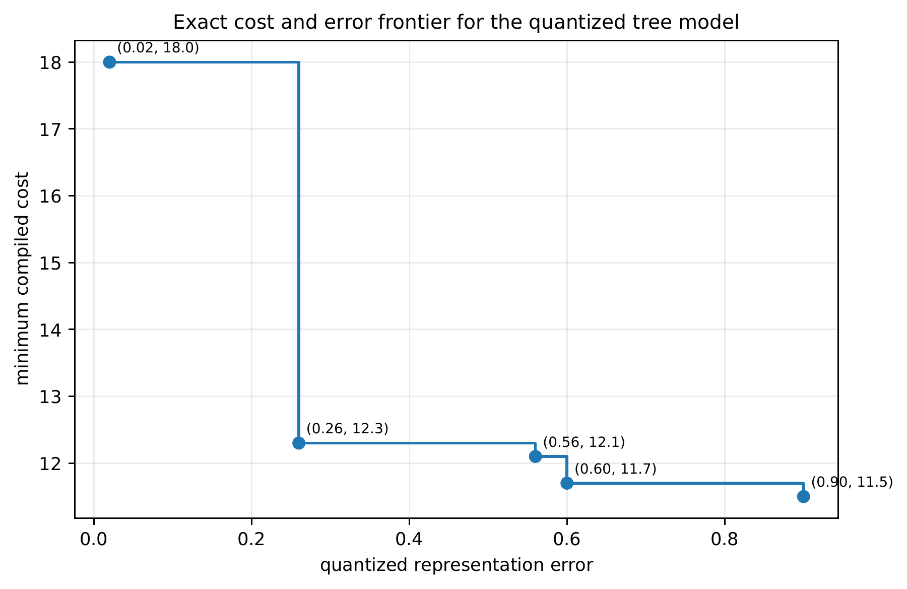
\[ ({\operatorname{cost}},{\operatorname{err}}). \]

The quantized budget compiler may recover Pareto points that are not optimal for any Lagrangian parameter.

Read proof · Visual guide: A penalty can miss the budget optimum · Read statement and proof side by side · Permalink · Source line 1643 · Claim record · Lean coverage · Code · Worked examples

Proof of Corollary 9.7

If another pruning had no larger cost and no larger error, with one strict inequality, its Lagrangian objective would be smaller. This contradicts optimality. A finite nonconvex frontier can contain points that are not supported by a line of slope \(-\lambda\), so the budget formulation is genuinely additional.

Back to statement · Read statement and proof side by side · Permalink · Source line 1651 · Claim record · Lean coverage · Code · Worked examples

9.3 An exact error budget compiler

On this page · Permalink · Source line 1655

Theorem 9.8: Quantized budget dynamic program

Assume every keep error is a nonnegative integer \(w_v\). Let \(B\in{\mathbb N}\). For each node \(v\), define \(F_v(b)\) as the minimum cost of a pruning of the subtree at \(v\) with total error exactly \(b\). The keep option contributes

\[ F_v(w_v)\leq\kappa_v. \]

The split option is obtained by min plus convolution of the child tables, followed by addition of \(\sigma_v\). The smallest value among

\[ F_{\rm root}(b), \qquad 0\leq b\leq B, \]

is the exact minimum cost among prunings whose quantized error is at most \(B\).

Read proof · Visual guide: A penalty can miss the budget optimum · Visual guide: Safe integers can still be conservative · Read statement and proof side by side · Permalink · Source line 1657 · Claim record · Lean coverage · Code · Worked examples

Proof of Theorem 9.8

The keep case is immediate. In the split case, an admissible pruning is the union of one admissible pruning from each child. Its error is the sum of the child errors and its cost is the sum of their costs plus \(\sigma_v\). Repeated min plus convolution enumerates every possible distribution of the integer budget across the child subtrees. Induction on the tree proves exactness.

Back to statement · Read statement and proof side by side · Permalink · Source line 1671 · Claim record · Lean coverage · Code · Worked examples

Corollary 9.9: Pseudo polynomial complexity

If the maximum number of children is bounded and the budget is \(B\), the quantized compiler has pseudo polynomial complexity in the number of tree nodes and \(B\). A direct pairwise convolution implementation has quadratic dependence on \(B\) at each merge.

Read proof · Visual guide: Safe integers can still be conservative · Read statement and proof side by side · Permalink · Source line 1675 · Claim record · Lean coverage · Code · Worked examples

Proof of Corollary 9.9

Every table has at most \(B+1\) entries. Merging two tables by direct convolution examines at most \((B+1)^2\) pairs. A bounded number of merges occurs at every node.

Back to statement · Read statement and proof side by side · Permalink · Source line 1679 · Claim record · Lean coverage · Code · Worked examples

The quantized dynamic program produces the exact cost and error frontier for its finite model.

9.4 Decision stability and local updates

On this page · Permalink · Source line 1690

Definition 9.10: Decision gap

At an internal node \(v\), let

\[ g_v = {\left\lvert K_\lambda(v)-S_\lambda(v)\right\rvert}. \]

This is the gap between the keep and split scores after the child subproblems have been solved.

Permalink · Source line 1692 · Claim record · Lean coverage · Code · Worked examples

Theorem 9.11: Compiler stability

Suppose the solved keep score and split score at every internal node change in absolute value by less than \(g_v/2\). These are scores after child subproblems have been solved, rather than unconstrained changes in raw local costs. Then every strict keep or split decision in the original optimal pruning remains unchanged.

Read proof · Visual guide: Recompile the changed part, not everything · Read statement and proof side by side · Permalink · Source line 1702 · Claim record · Lean coverage · Code · Worked examples

Proof of Theorem 9.11

If the original keep score is lower by \(g_v\), then after perturbation it can increase by less than \(g_v/2\), while the split score can decrease by less than \(g_v/2\). The order remains strict. The split case is the same. Apply the argument from the leaves upward.

Back to statement · Read statement and proof side by side · Permalink · Source line 1706 · Claim record · Lean coverage · Code · Worked examples

Theorem 9.12: Local recompilation

Suppose local costs change only inside the subtree rooted at \(u\), while ancestor and sibling local models are unchanged. Use correct cached sibling values from the old solve. Then every dynamic programming value outside that subtree and outside the ancestor chain from \(u\) to the root remains unchanged. Recomputing the subtree at \(u\) and that ancestor chain gives the exact new global optimum.

Read proof · Visual guide: Recompile the changed part, not everything · Read statement and proof side by side · Permalink · Source line 1710 · Claim record · Lean coverage · Code · Worked examples

Proof of Theorem 9.12

A node value depends only on its own local data and the values of its children. Nodes outside the changed subtree and outside the ancestor chain have the same local data and the same child values. Their values remain unchanged. Every affected dependency lies inside the changed subtree or on the unique path from \(u\) to the root.

Back to statement · Read statement and proof side by side · Permalink · Source line 1714 · Claim record · Lean coverage · Code · Worked examples

Remark 9.13: Boundary of the compiler theorem

The exact compiler requires a finite candidate tree and additive local models. Arbitrary overlapping decompositions, nonlocal cache interactions, global rank coupling, and unrestricted structure discovery can destroy optimal substructure. No universal approximation factor is proved for those settings.

Permalink · Source line 1718

Source and conversion record

Source SHA-256: ef616bca9291ac766d492b88f3166be4bc2b39f9ba6034dea3a4bcf2d2bf5d7f

Unsupported prose commands stop the build. The mathematical expression sequence is checked against the source, with manuscript macros expanded for display.

Conversion records

Read and explore

Proofs and implementation

About this work

Other resources