12 Recorded CPU and GPU corpus
On this page · Visual guide: Same output before comparing times · Permalink · Source line 1857
The empirical corpus contains 154 measured rows from sixteen suites. It has 74 CPU rows and 80 GPU rows. The GPU was an NVIDIA GeForce RTX 3070 Ti Laptop GPU with compute capability 8.6 and 8 GB nominal memory. The recorded software used PyTorch 2.11.0 with a CUDA 12.8 build. These facts identify the environment. They do not predict another machine.
| Suite | Rows | Suite | Rows |
|---|---|---|---|
| Dense multiplication | 28 | BDLR application | 15 |
| Block diagonal | 12 | BDLR product | 12 |
| Circulant | 12 | Toeplitz | 12 |
| Kronecker | 12 | Block banded | 8 |
| Sparse plus low rank | 8 | HODLR | 8 |
| Strassen | 6 | Transfer pipeline | 5 |
| Walsh Hadamard | 4 | Hidden blocks | 4 |
| Randomized low rank | 4 | Iterative refinement | 4 |
The 154 archived rows contain recorded case identifiers, seeds, types, output contracts, and timing scopes. Source-value hashes and explicit correctness-reference fields are absent. Setup time, discovery time, and reuse count are nonnull in only two rows each; correctness errors are present in 149 rows. Equality of available metadata cannot establish the full fair-match relation in Definition 11.2. In particular, CPU-resident and GPU-device-resident scopes differ, and graph replay excludes capture while a device-resident baseline has a different raw scope. The two-stream example also compares wall time with a serial device-time scope. The values below are retained as historical observations with these limitations.
12.1 Dense precision frontier
On this page · Permalink · Source line 1884
At dimension \(4096\), the device resident dense rows gave the values in Table 2.
| Method | Median time in ms | Logical GFLOP per second | Relative error |
|---|---|---|---|
| FP64 | 541.2803 | 253.91 | \(2.18\times10^{-15}\) |
| FP32 | 18.1309 | 7580.35 | \(5.76\times10^{-7}\) |
| TF32 | 8.6999 | 15797.75 | \(2.94\times10^{-4}\) |
| FP16 | 4.0264 | 34134.72 | \(3.60\times10^{-4}\) |
| BF16 | 4.1482 | 33132.00 | \(2.88\times10^{-3}\) |
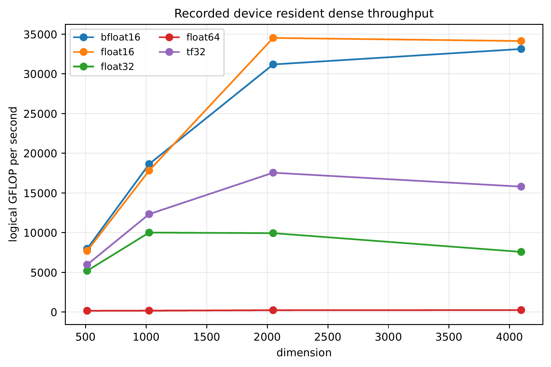
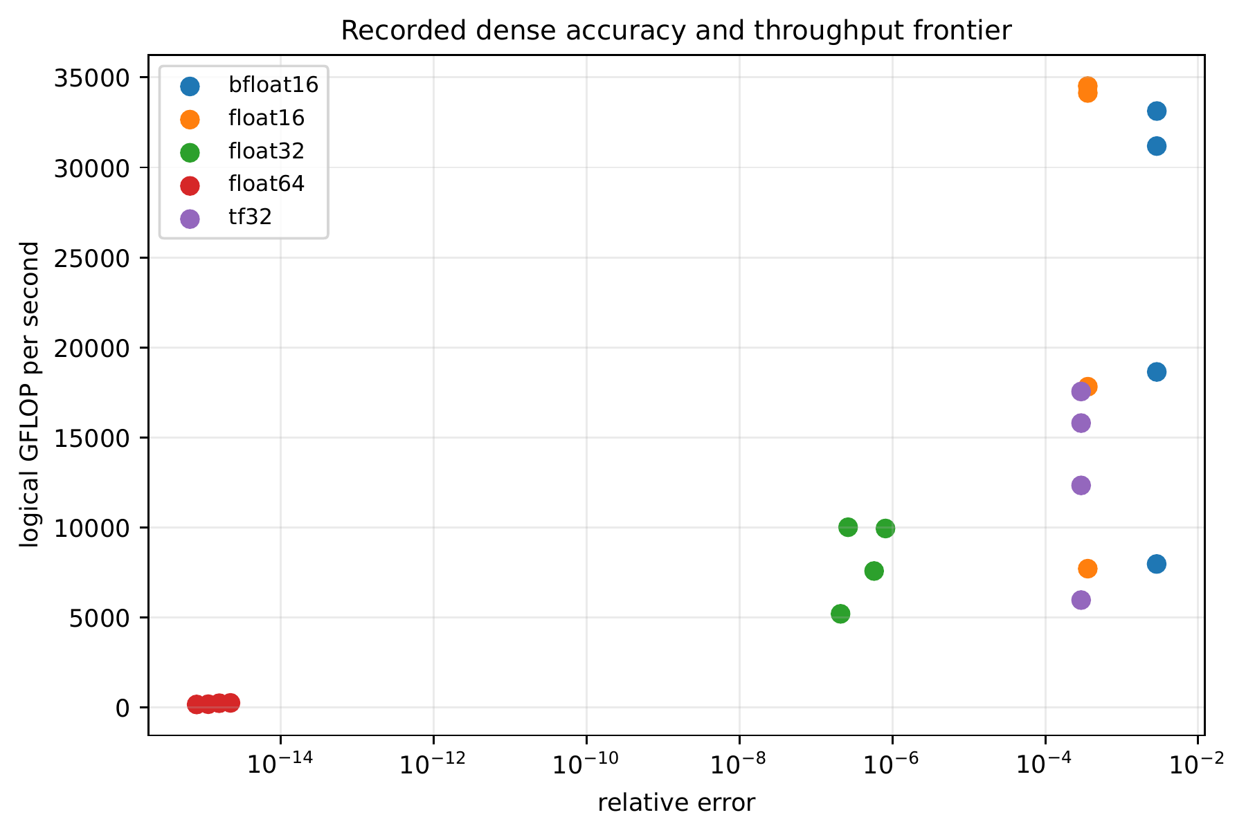
The frontier is not a universal ordering of scalar types. It records one generated family. Packet precision assignment should use local sensitivities and supported kernels rather than one global type.
12.2 Regular packet operators
On this page · Permalink · Source line 1922
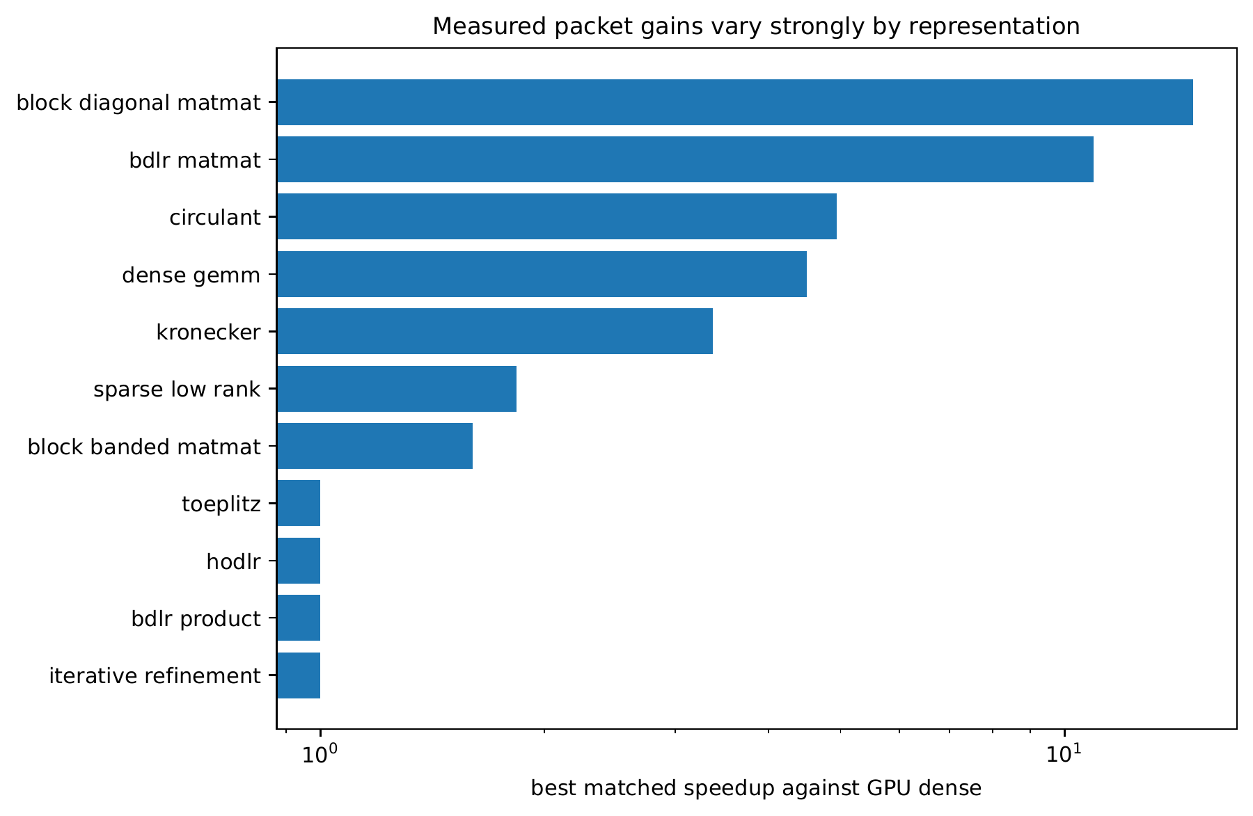
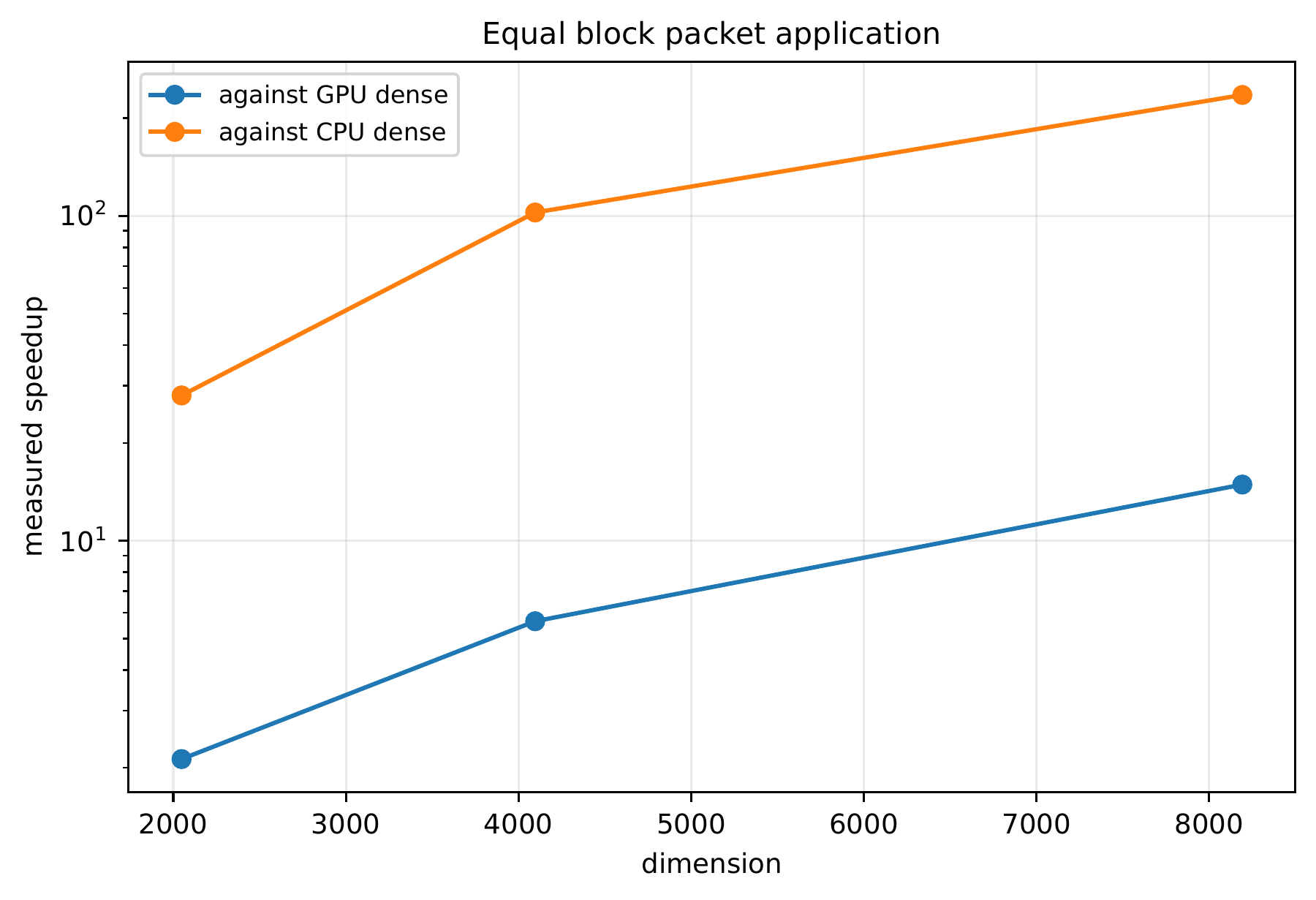
For an \(8192\) by \(8192\) equal block operator with block width \(64\) and \(32\) right hand sides, the batched packet calculation took
It was
times faster than the recorded device resident dense GPU row with the same recorded case, output, and timing scope and
times faster than the recorded CPU dense row (resident CPU scope versus device-resident GPU scope). The relative error was
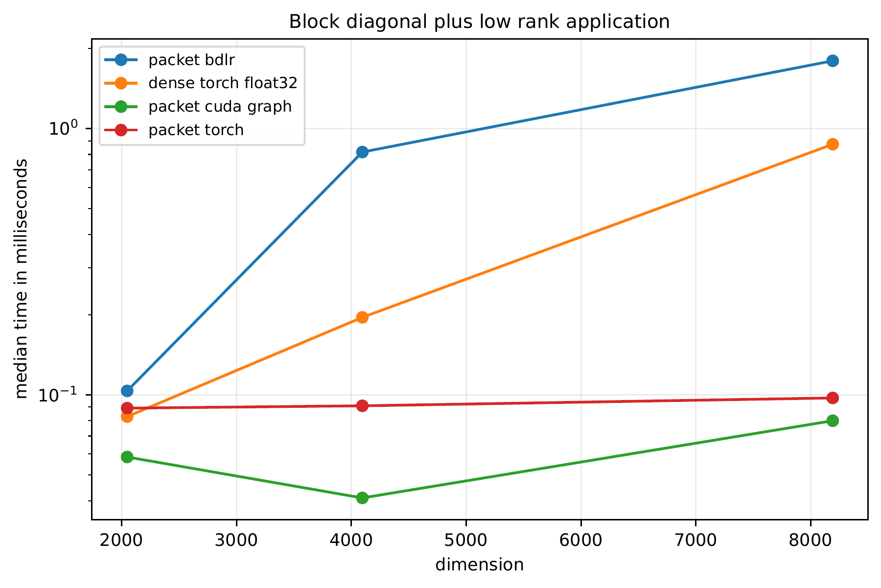
For BDLR application with the same dimension and right hand side count, block width \(64\), and rank \(8\), CUDA Graph replay took
It was
times faster than the recorded dense GPU row (graph-replay scope versus device-resident scope) and
times faster than the recorded CPU dense row (resident CPU scope versus device-resident GPU scope). Capture time was excluded from the replay scope and must be amortized separately.
12.3 Compressed products
On this page · Permalink · Source line 1969
A compressed BDLR product returns block and low rank factors. Materialization returns all matrix entries. The historical product rows illustrate the cost of changing the output contract; compressed and materialized outputs are separate computations. The GPU materialized BDLR rows at dimensions 512 and 1024 are sums of separately measured factor and expansion medians, as the raw notes state; they are not complete-workflow timing medians.
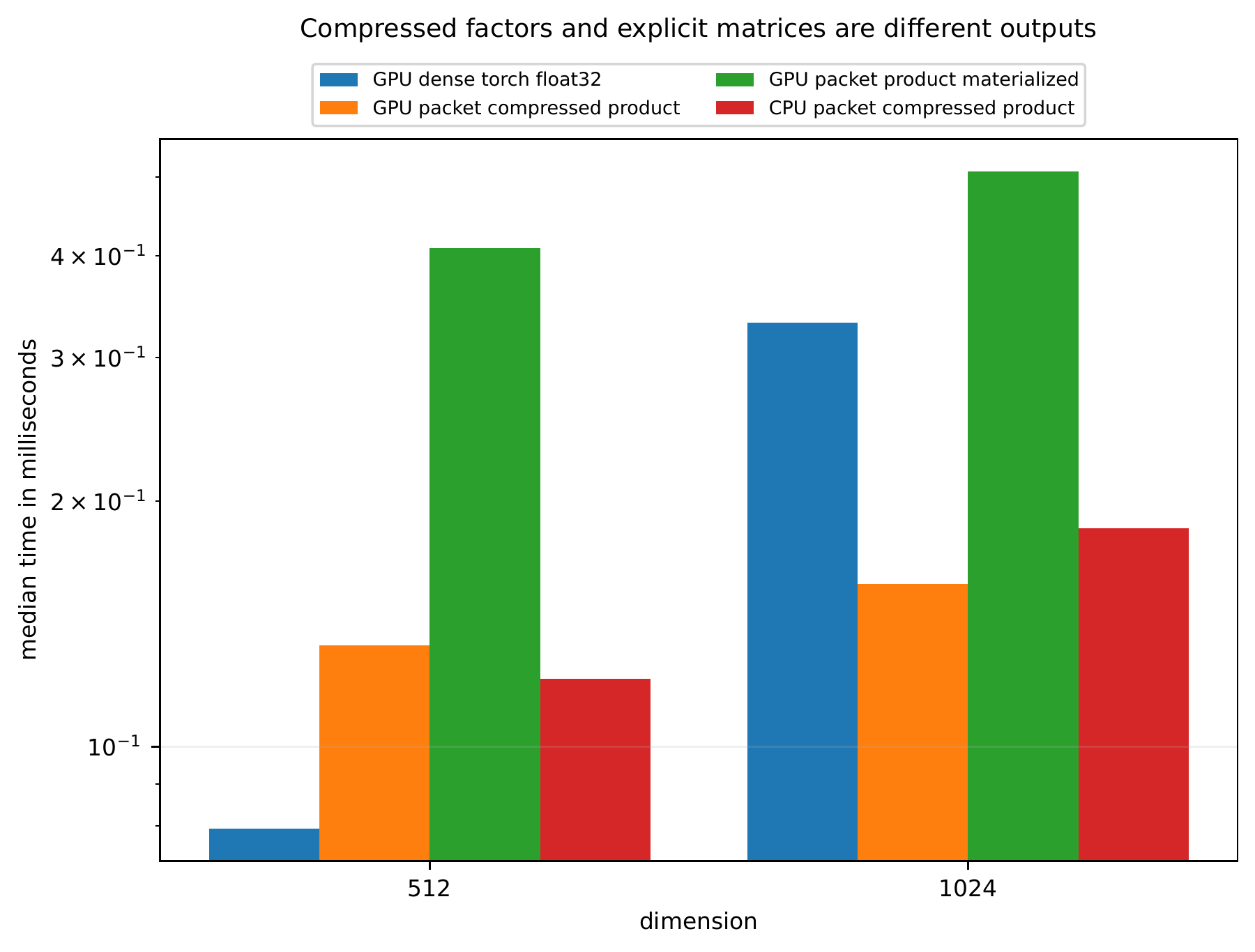
The algebra in Theorem 5.1 explains why the compressed product can remain small. The materialization cost in Proposition 3.10 explains why explicit output can erase the advantage.
12.4 Discovery and transfer
On this page · Permalink · Source line 1982
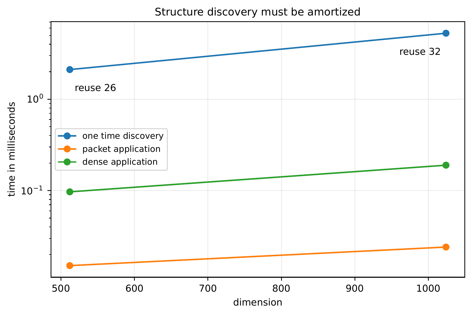
For hidden permuted blocks at dimension \(512\), structure discovery took \(2.1102\) ms, dense application took \(0.0969\) ms, and packet application took \(0.0151\) ms. The exact threshold in Theorem 10.4 is \(26\) uses. At dimension \(1024\), the corresponding values were \(5.2726\), \(0.1896\), and \(0.0241\) ms, giving \(32\) uses.
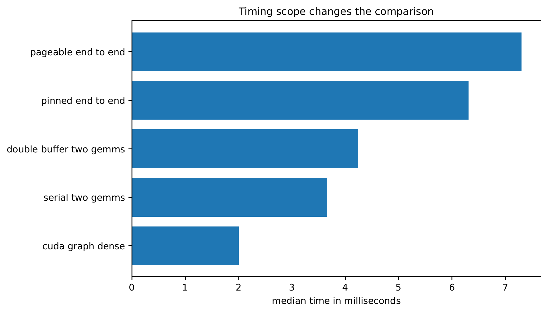
For one \(2048\) dense FP32 product, device resident graph replay took \(1.9993\) ms. The end to end pageable path took \(7.3036\) ms. The pinned path took \(6.3084\) ms. Two serial device resident products took \(3.6557\) ms, while the tested two stream path took \(4.2368\) ms.
12.5 Negative controls
On this page · Permalink · Source line 2002
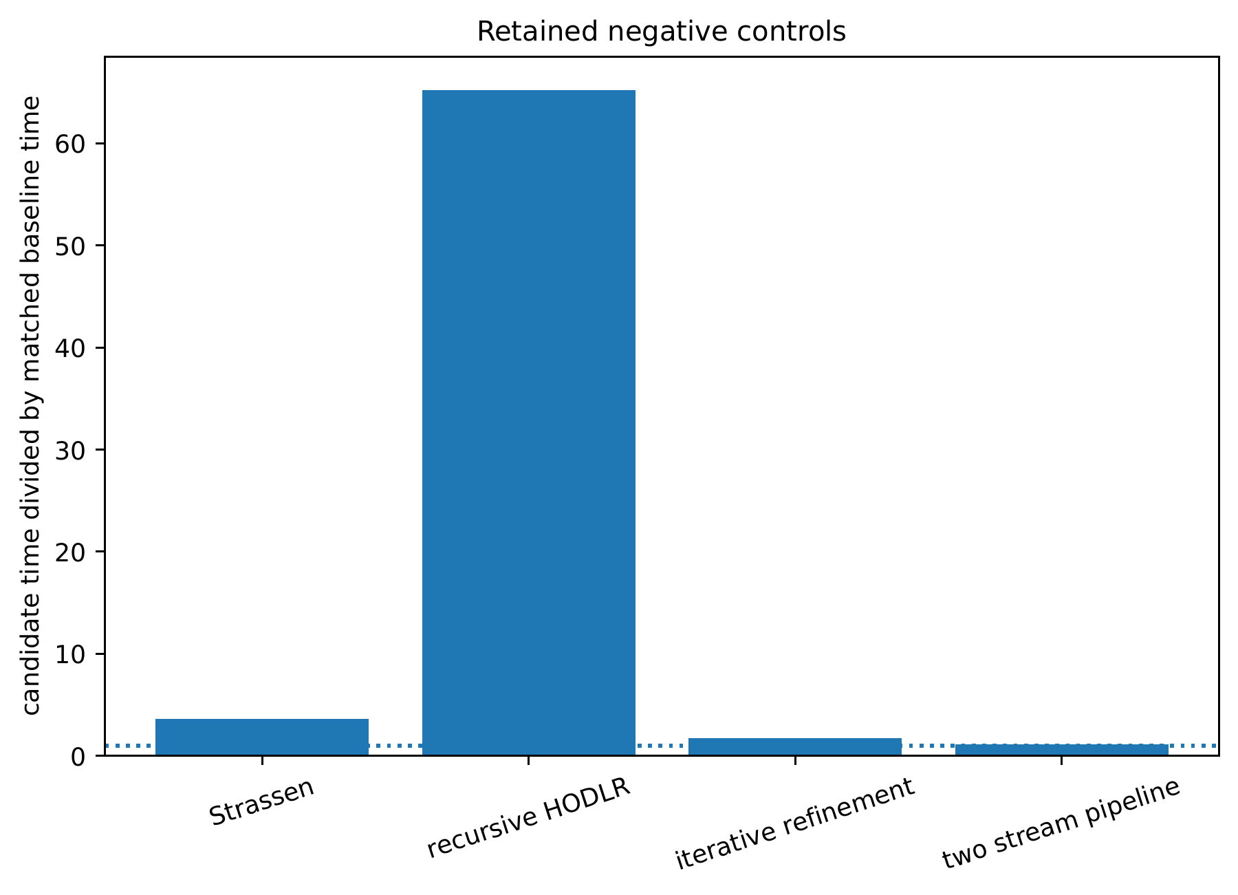
The corpus retains methods that lost in the recorded baseline comparisons. These are descriptive ratios; scope and complete-metadata qualifications apply.
At dimension \(512\), recursive Strassen multiplication with leaf size \(128\) took \(7.0950\) ms, while the recorded OpenBLAS dense multiplication took \(1.9597\) ms.
At dimension \(2048\), the tested recursive HODLR GPU path took \(5.6079\) ms, while dense GPU multiplication took \(0.0860\) ms.
The tested FP32 iterative refinement solve took \(22.0848\) ms, while the direct FP64 GPU solve took \(12.6286\) ms with a comparable final error.
The two stream dense path was slower than the serial two product path.
The GPU Walsh Hadamard transform was slower than the CPU implementation at length \(65536\), then became faster at length \(262144\).
Fast multiplication can be asymptotically valuable and still lose at measured sizes because of recursion, memory traffic, and kernel granularity. Hierarchical matrix methods have similar crossover issues [AmbikasaranDarve2013]. Transform algorithms and tensor factorizations form additional structure classes [CooleyTukey1965], [Oseledets2011].