
Three exact models before the general theory
On this page · Permalink · Source line 2
These models use exact integers and rational numbers. Their costs and integer errors are declared illustrative quantities. The figures display the computed records. They do not report timings or identify actual hardware precision types.
A low rank action and its inverse
On this page · Permalink · Source line 6
Set
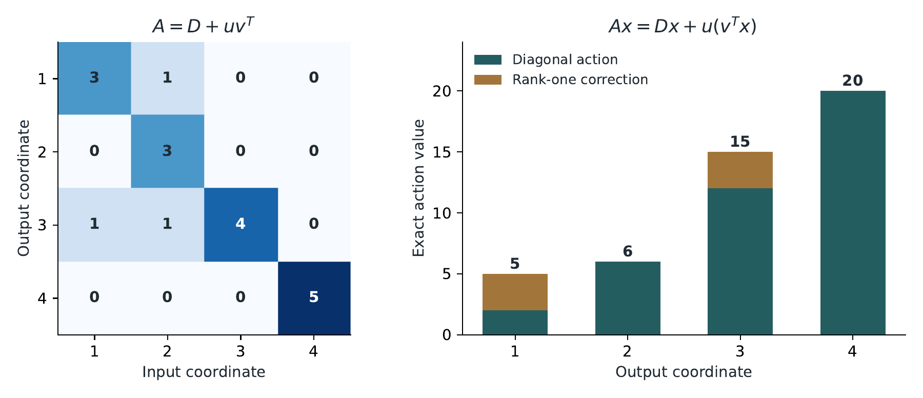
and define \(A=D+uv^T\). Its entries are shown in the figure. The same operator can be stored by its diagonal and two thin vectors rather than by every matrix entry. For \(x=(1,2,3,4)^T\), first form \(v^Tx=3\). Then
so \(Ax=(5,6,15,20)^T\). Only the first and third output coordinates receive the correction.
The inverse starts with the same representation. Write \(y=Ax\). Since \(D\) is invertible,
The scalar Woodbury core is therefore invertible. Its correction coefficient is
Subtracting that correction recovers the original input:
What the output contract preserves
The diagonal and thin vectors use twelve scalar slots, compared with sixteen for the explicit matrix. This small storage count assumes the full thin vectors are stored. It does not predict elapsed time. A compressed action returns \(Ax\). Materializing all entries of \(A\) produces another output and incurs its own work. The general formulas appear in Theorem 2.3 and Theorem 5.3.
A budget can select a point that no Lagrangian selects
On this page · Permalink · Source line 46
Consider a rooted candidate tree. The root \(r\) has children \(a,b\), and \(a\) has children \(a_1,a_2\). Split overheads are zero. Each retained node has the following declared cost and integer error:
| Node | \(r\) | \(a\) | \(b\) | \(a_1\) | \(a_2\) |
|---|---|---|---|---|---|
| Cost | 1 | 2 | 1 | 3 | 1 |
| Error | 6 | 4 | 0 | 1 | 0 |
Exactly three prunings are possible:
| Selected nodes | Total cost | Total error |
|---|---|---|
| \(r\) | 1 | 6 |
| \(a,b\) | 3 | 4 |
| \(a_1,a_2,b\) | 5 | 1 |
For a Lagrangian multiplier \(\lambda\ge0\), their objectives are \(1+6\lambda\), \(3+4\lambda\), and \(5+\lambda\). The middle pruning can be optimal only if
These inequalities require \(\lambda\ge1\) and \(\lambda\le2/3\) simultaneously. There is no such multiplier. The root and full split exchange optimality at \(\lambda=4/5\), where both have objective \(29/5\).
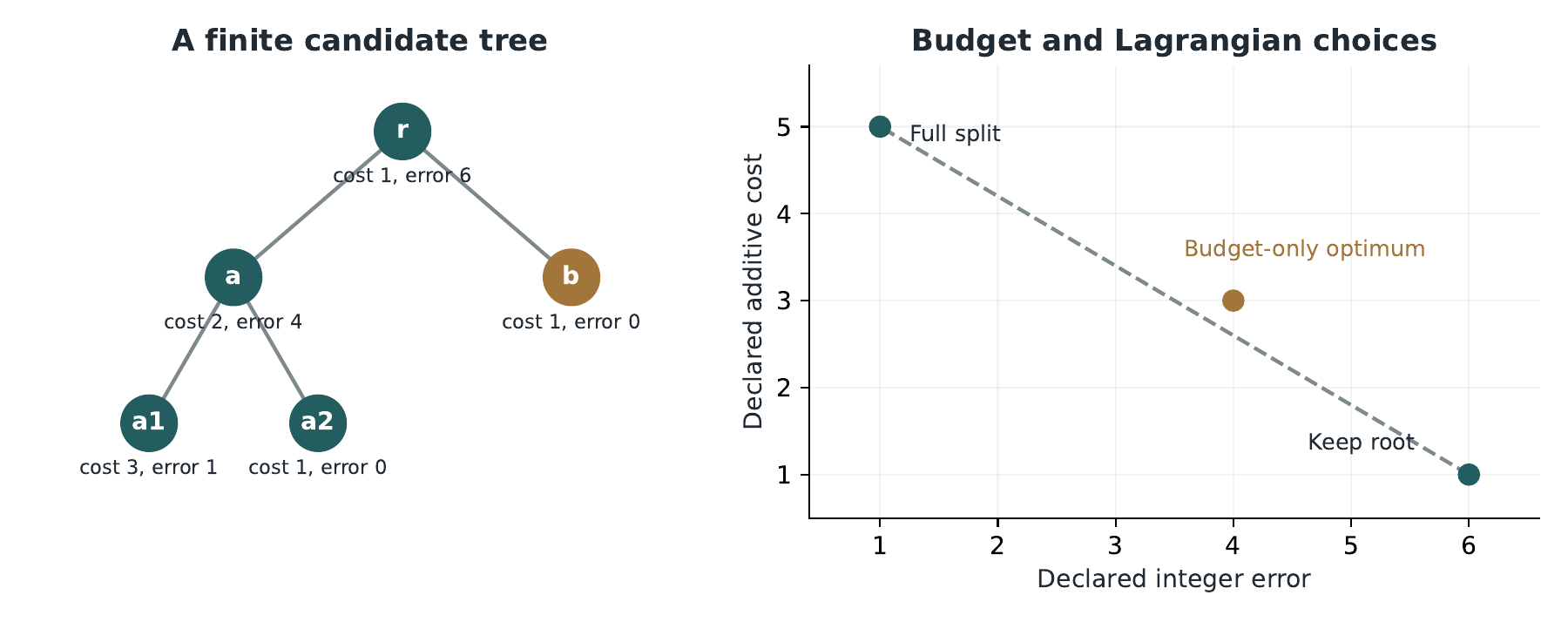
The budget problem still selects that middle pruning. Under the constraint \({\operatorname{err}}\le4\), the root is infeasible. The two feasible costs are three and five, so the minimum is three. Under budget one, only the full split is feasible. Under budget six, the root is cheapest. Thus the budget program adds something that changing \(\lambda\) cannot recover.
The dynamic recurrence gives the same Lagrangian choices without listing prunings. At \(a\), it compares \(2+4\lambda\) with \(4+\lambda\). At \(r\), it compares \(1+6\lambda\) with \(1+F_\lambda(a)\). Its exactness follows from the finite tree and additive model in Theorem 9.4 and Theorem 9.8. Overlapping decompositions or nonlocal execution costs need another argument.
Discrete precision follows the sensitive edge
On this page · Permalink · Source line 82
Suppose three packet edges each admit a fast option F and an accurate option A. The names describe the supplied model, rather than any actual scalar type. Exactly one option is chosen on each edge:
| F | A | |||
|---|---|---|---|---|
| Edge | Cost | Error | Cost | Error |
| 1 | 1 | 5 | 4 | 0 |
| 2 | 1 | 2 | 3 | 0 |
| 3 | 1 | 1 | 3 | 0 |
The all-fast assignment FFF has cost three and error eight. It exceeds budget three. Changing only edge one to A gives AFF, with cost \(4+1+1=6\) and error \(0+2+1=3\). Changing only edges two and three gives FAA, with cost seven and error five. That choice still exceeds the budget.
All eight assignments can be checked directly:
| Assignment | Cost | Error | Assignment | Cost | Error |
|---|---|---|---|---|---|
| FFF | 3 | 8 | AFF | 6 | 3 |
| FFA | 5 | 7 | AFA | 8 | 2 |
| FAF | 5 | 6 | AAF | 8 | 1 |
| FAA | 7 | 5 | AAA | 10 | 0 |
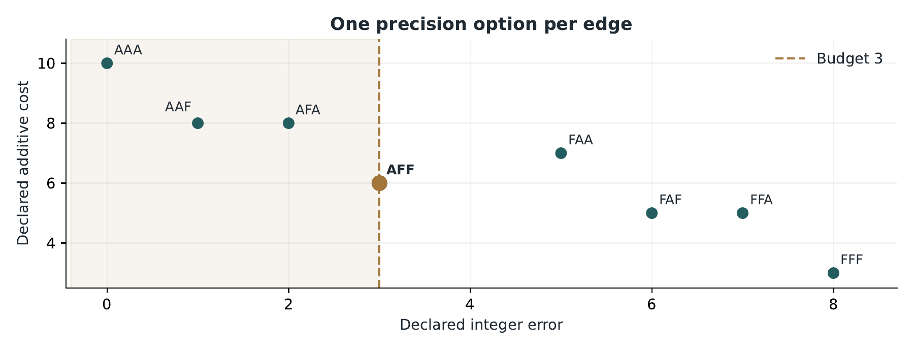
The exact recurrence reaches the same result. After edge one, only \(({\operatorname{err}},{\operatorname{cost}})=(5,1)\) and \((0,4)\) are reachable. After edge two, the reachable states are \((7,2)\), \((5,4)\), \((2,5)\), and \((0,7)\). Extending these with either option on edge three gives the final eight assignments. Among states of error at most three, the lowest cost is six.
The certificate belongs to the model
The integer error weights must be supplied by a stated certificate or quantization rule. The recurrence solves that finite model exactly. Kernel accumulation, overflow, underflow, scaling, and shape support require their own assumptions before an actual implementation can use the result. The precise recurrence is Theorem 8.7.
The complete rational records, dynamic tables, and five rejected false controls are reproduced by generate_monograph_examples.py. Figure generation converts those records to plotting coordinates only after the exact checks pass.