
Reading the figure
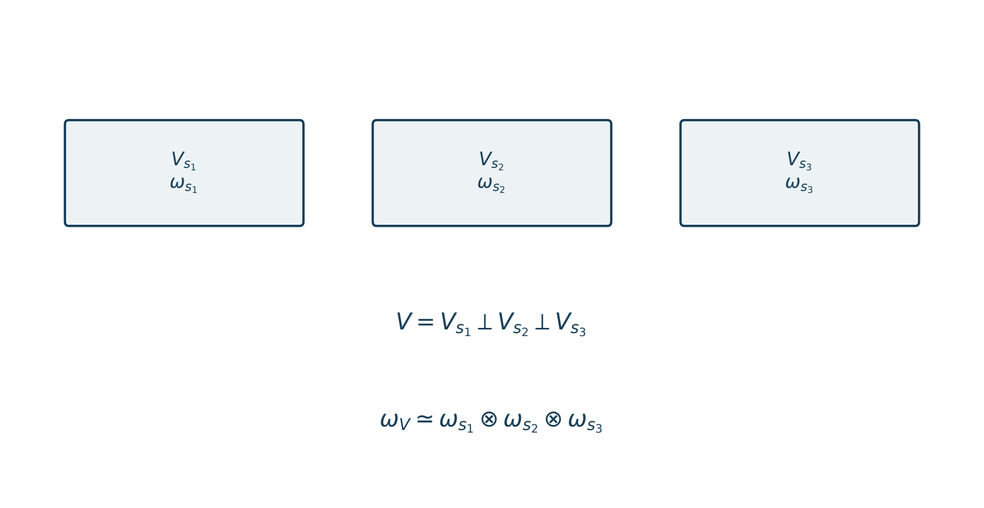
Three break spaces and their representations appear above an orthogonal decomposition and its tensor-product representation. The source gives the hypotheses for that factorization.
Mathematical labels
\(V=V_{s_1}\perp V_{s_2}\perp V_{s_3}\)
\(\omega_V\simeq\omega_{s_1}\otimes\omega_{s_2}\otimes\omega_{s_3}\)
Selectable labels from the original PDF
Native PDF text retains the figure’s extraction order. Equations and data tables above provide the reading order.
Vs1
ωs1
Vs2
ωs2
Vs3
ωs3
V = Vs1 ⟂ Vs2 ⟂ Vs3
ωV ≃ ωs1 ⊗ ωs2 ⊗ ωs3
Original figure caption
Symplectic direct sum and Heisenberg tensor product are compatible.
For \(V=\perp_sV_s\) and compatible central characters,
The groups combine by a central product. Tensoring the individual intertwiners gives the full finite bridge, once the stabilizer actions and phases agree. Transport-graph compatibility is then the matrix holonomy condition.
Scope
Separate actual type quotients at each break do not, merely by tensoring, become one actual maximal simple type in the source atom's rank. Constructing a common arithmetic carrier and recovering a candidate are the extra realization requirements.