
Reading the figure
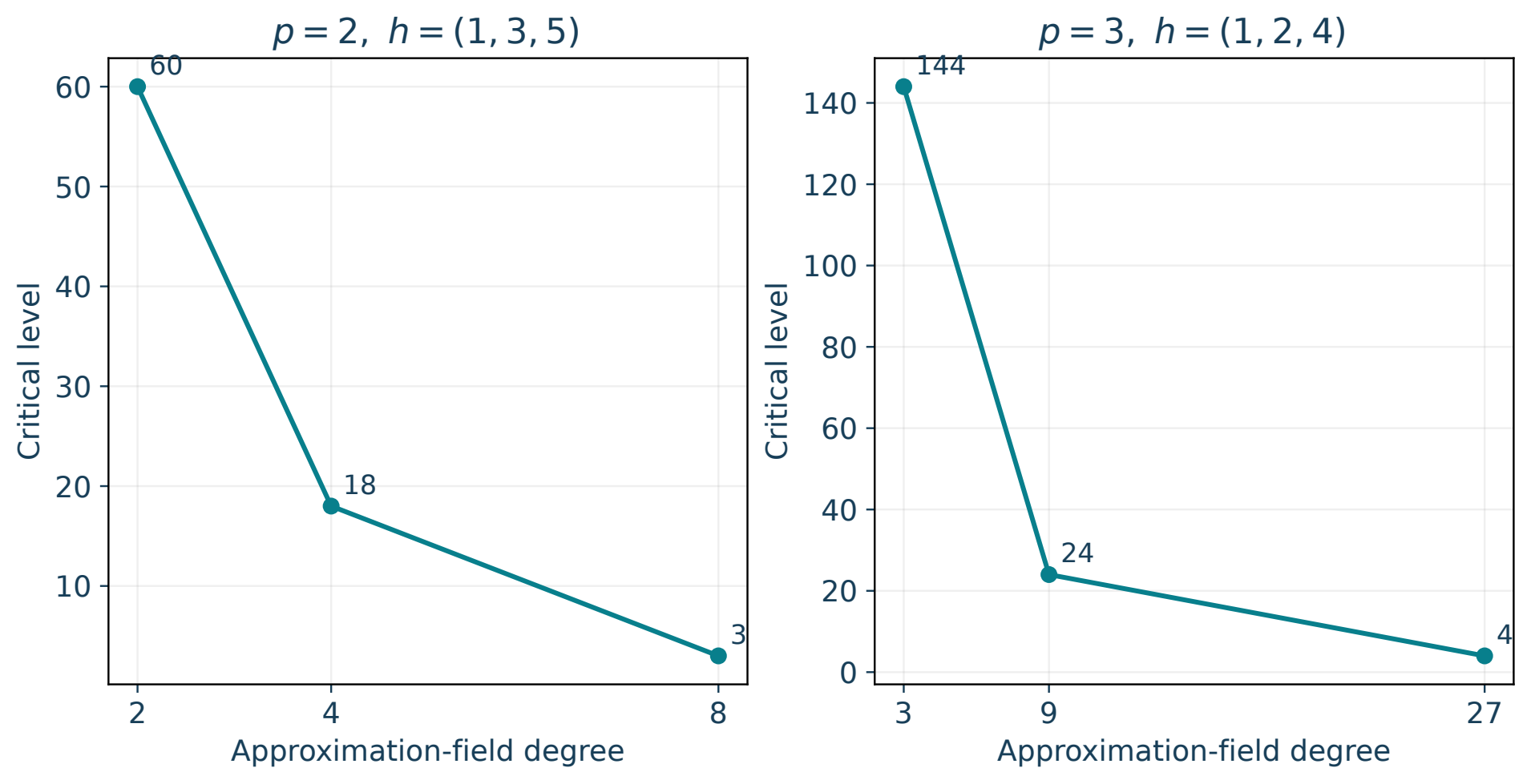
The dyadic example uses degrees two, four and eight with levels sixty, eighteen and three. The odd example uses degrees three, nine and twenty-seven with levels one hundred forty-four, twenty-four and four. These are finite illustrative profiles.
Mathematical labels
\(p=2,\ h=(1,3,5)\)
\(p=3,\ h=(1,2,4)\)
| Stage | Dyadic level | Odd p = 3 level |
|---|---|---|
| 1 | 60 | 144 |
| 2 | 18 | 24 |
| 3 | 3 | 4 |
Selectable labels from the original PDF
Native PDF text retains the figure’s extraction order. Equations and data tables above provide the reading order.
2 4 8
Approximation-field degree
10
20
30
40
50
60
Critical level
60
18
3
p = 2, h = (1, 3, 5)
3 9 27
Approximation-field degree
0
20
40
60
80
100
120
140
Critical level
144
24
4
p = 3, h = (1, 2, 4)
Original figure caption
These examples were recomputed exactly; the all-length assertions are proved separately.
For increasing permitted \(h_1<\cdots<h_d\), put \(q_i=(p+1)h_i\) and \(N=p^d\). The approximation-field degrees are \(p,p^2,\ldots,p^d\), with
For odd \(p\), require \(p\nmid h_i\). For \(p=2\), require all \(h_i\) odd and positive. The leading ambient level is \(n_1\); \(n_2,\ldots,n_d\) are the successive critical approximation levels.
Scope
Every amplified ambient approximation still has leading level \(n_1\). The declining values plotted here are critical levels, not new leading valuations for those ambient matrices.