Paper II: Refinement and residue coordinates

3 Packet systems and refinement towers

On this page · Permalink · Source line 1

Packet coordinates split a module into pieces that can be recovered separately and then added back together. The construction uses idempotents and does not need an inner product.

Permalink · Source line 3

Definition 3.1: Packet system

Let \(X\) be a module over a unital ring. A finite packet system on \(X\) is a family

\[ {\mathcal P}=(P_\alpha)_{\alpha\in I} \subseteq{\operatorname{End}}(X) \]

of nonzero idempotents such that

\[ P_\alpha P_\beta=0 \quad\text{when }\alpha\ne\beta, \qquad \sum_{\alpha\in I}P_\alpha=I_X. \]

Write

\[ X_\alpha=P_\alpha X, \qquad X^{{\mathcal P}}=\bigoplus_{\alpha\in I}X_\alpha. \]

The analysis and synthesis maps are

\[ {\mathcal A}_{{\mathcal P}}x=(P_\alpha x)_\alpha, \qquad {\mathcal S}_{{\mathcal P}}(x_\alpha)_\alpha=\sum_\alpha x_\alpha. \]

They are inverse isomorphisms.

Permalink · Source line 5 · Claim record · Lean coverage · Code · Worked examples

Definition 3.2: Refinement

Let \({\mathcal P}=(P_\alpha)_{\alpha\in I}\) and \({\mathcal Q}=(Q_\beta)_{\beta\in J}\) be packet systems on the same module. We say that \({\mathcal Q}\) refines \({\mathcal P}\) when there is a surjection

\[ \rho:J\longrightarrow I \]

such that

\[ P_\alpha=\sum_{\rho(\beta)=\alpha}Q_\beta \]

for every \(\alpha\in I\). The index \(\beta\) is then called a child of \(\rho(\beta)\).

Visual guide: An atlas of the refinement layer · Permalink · Source line 33 · Claim record · Lean coverage · Code · Worked examples

Theorem 3.3: Children, parents, and transitivity

Suppose that \({\mathcal Q}\) refines \({\mathcal P}\) through \(\rho\). Then

\[ P_\alpha Q_\beta = Q_\beta P_\alpha = \begin{cases} Q_\beta & \rho(\beta)=\alpha,\\ 0 & \rho(\beta)\ne\alpha. \end{cases} \]

Hence \(Q_\beta X\subseteq P_{\rho(\beta)}X\). If a third packet system \({\mathcal R}\) refines \({\mathcal Q}\), then \({\mathcal R}\) refines \({\mathcal P}\) through the composite parent map.

Read proof · Visual guide: Follow one coefficient through the tower · Read statement and proof side by side · Permalink · Source line 45 · Claim record · Lean coverage · Code · Worked examples

Proof of Theorem 3.3

Multiply the identity

\[ P_\alpha=\sum_{\rho(\gamma)=\alpha}Q_\gamma \]

by \(Q_\beta\) on either side. Pairwise annihilation in the fine family leaves \(Q_\beta\) when \(\rho(\beta)=\alpha\) and leaves zero otherwise. For transitivity, substitute the child expansion of each \(Q_\beta\) into the expansion of \(P_\alpha\) and group the resulting terms by the composite parent.

Back to statement · Read statement and proof side by side · Permalink · Source line 60 · Claim record · Lean coverage · Code · Worked examples

A refinement tower is a sequence \(({\mathcal P}_\ell)_{\ell\geq0}\) with parent maps

\[ \rho_{m,\ell}:I_m\longrightarrow I_\ell \qquad(m\geq\ell) \]

such that \({\mathcal P}_m\) refines \({\mathcal P}_\ell\) through \(\rho_{m,\ell}\) for every \(m\geq\ell\), and

\[ \rho_{\ell,\ell}={\mathrm{id}}_{I_\ell}, \qquad \rho_{n,\ell}=\rho_{m,\ell}\circ\rho_{n,m} \qquad(n\geq m\geq\ell). \]

Thus every parent map witnesses the stated refinement and the maps compose coherently. The next result shows that the coordinate changes form a coherent system.

Permalink · Source line 68

Definition 3.4: Coordinate change across levels

For two packet systems \({\mathcal P}\) and \({\mathcal Q}\) on \(X\), define

\[ J_{{\mathcal Q}\leftarrow{\mathcal P}} = {\mathcal A}_{{\mathcal Q}}{\mathcal S}_{{\mathcal P}}:X^{{\mathcal P}}\longrightarrow X^{{\mathcal Q}} \]

and

\[ C_{{\mathcal P}\leftarrow{\mathcal Q}} = {\mathcal A}_{{\mathcal P}}{\mathcal S}_{{\mathcal Q}}:X^{{\mathcal Q}}\longrightarrow X^{{\mathcal P}}. \]

When \({\mathcal Q}\) refines \({\mathcal P}\), the first map resolves each coarse coordinate into its children and the second adds the children back to their parent.

Visual guide: Three kinds of resolution · Visual guide: An atlas of the refinement layer · Visual guide: Regrouping is not averaging · Permalink · Source line 82 · Claim record · Lean coverage · Code · Worked examples

The central idea

A coarse coordinate retains a whole vector in its coarse packet. Adding its children keeps the whole vector inside that packet. Fine analysis recovers each child by applying its projector. This explains why the two coordinate maps can be inverse even when the fine system has more packet labels.

Permalink · Source line 98

Theorem 3.5: Exact coordinate change and coherence

For any two packet systems on \(X\),

\[ C_{{\mathcal P}\leftarrow{\mathcal Q}}J_{{\mathcal Q}\leftarrow{\mathcal P}}=I_{X^{{\mathcal P}}}, \qquad J_{{\mathcal Q}\leftarrow{\mathcal P}}C_{{\mathcal P}\leftarrow{\mathcal Q}}=I_{X^{{\mathcal Q}}}. \]

For three packet systems \({\mathcal P}\), \({\mathcal Q}\), and \({\mathcal R}\) on \(X\),

\[ J_{{\mathcal R}\leftarrow{\mathcal Q}}J_{{\mathcal Q}\leftarrow{\mathcal P}} = J_{{\mathcal R}\leftarrow{\mathcal P}}, \]

\[ C_{{\mathcal P}\leftarrow{\mathcal Q}}C_{{\mathcal Q}\leftarrow{\mathcal R}} = C_{{\mathcal P}\leftarrow{\mathcal R}}. \]

If \({\mathcal Q}\) refines \({\mathcal P}\) through \(\rho\), then

\[ \bigl(J_{{\mathcal Q}\leftarrow{\mathcal P}}x\bigr)_\beta = Q_\beta x_{\rho(\beta)}, \qquad \bigl(C_{{\mathcal P}\leftarrow{\mathcal Q}}y\bigr)_\alpha = \sum_{\rho(\beta)=\alpha}y_\beta. \]

Read proof · Visual guide: Regrouping is not averaging · Visual guide: The operator changes coordinates too · Read statement and proof side by side · Permalink · Source line 102 · Claim record · Lean coverage · Code · Worked examples

Proof of Theorem 3.5

The packet analysis and synthesis maps are inverse. Therefore

\[ C_{{\mathcal P}\leftarrow{\mathcal Q}}J_{{\mathcal Q}\leftarrow{\mathcal P}} = {\mathcal A}_{{\mathcal P}}{\mathcal S}_{{\mathcal Q}}{\mathcal A}_{{\mathcal Q}}{\mathcal S}_{{\mathcal P}} = {\mathcal A}_{{\mathcal P}}{\mathcal S}_{{\mathcal P}} = I. \]

The other inverse identity is the same calculation with the two systems exchanged. The coherence identities follow by inserting

\[ {\mathcal S}_{{\mathcal Q}}{\mathcal A}_{{\mathcal Q}}=I_X. \]

Now assume that \({\mathcal Q}\) refines \({\mathcal P}\). If \(x=(x_\alpha)_\alpha\) with \(x_\alpha\in P_\alpha X\), then

\[ Q_\beta\sum_\alpha x_\alpha = Q_\beta x_{\rho(\beta)} \]

by Theorem 3.3. The formula for \(C\) follows by synthesis followed by projection onto the parent packet.

Back to statement · Read statement and proof side by side · Permalink · Source line 132 · Claim record · Lean coverage · Code · Worked examples

Remark 3.6: Refinement and reduction

The maps in Theorem 3.5 are isomorphisms because both coordinate spaces represent all of \(X\). They do not reduce dimension and they do not discard packets. Approximation begins only after one chooses a truncation or compression rule.

Permalink · Source line 156

Corollary 3.7: Orthogonal Hilbert packets

If \(X\) is a real or complex Hilbert space and every packet system in the tower consists of orthogonal projections, equip each finite packet direct sum with the Hilbert inner product \(\langle(x_\alpha),(y_\alpha)\rangle=\sum_\alpha\langle x_\alpha,y_\alpha\rangle\). Then analysis and synthesis are unitary. Every coordinate change in Theorem 3.5 is unitary.

Read proof · Read statement and proof side by side · Permalink · Source line 160 · Claim record · Lean coverage · Code · Worked examples

Proof of Corollary 3.7

For an orthogonal packet system,

\[ \|x\|^2=\sum_\alpha\|P_\alpha x\|^2. \]

Thus analysis is an isometry onto the full packet direct sum. Synthesis is its inverse. A coordinate change is a composition of two unitary maps.

Back to statement · Read statement and proof side by side · Permalink · Source line 164 · Claim record · Lean coverage · Code · Worked examples

Every coarse packet is also uniquely reconstructed from its fine children. If vectors \(x_\beta\in Q_\beta X\) sum to a coarse packet \(x\), applying \(Q_\gamma\) recovers \(x_\gamma=Q_\gamma x\). This is the uniqueness clause of the canonical nested-refinement statement.

Permalink · Source line 172

3.1 Typed coordinate naturality

On this page · Permalink · Source line 174

These coordinate changes are coherent through every finite tower. If three complete packet systems are denoted by \(a,b,c\), then

\[ J_{c,b}J_{b,a}=J_{c,a}, \qquad J_{a,a}=I, \qquad J_{b,a}^{-1}=J_{a,b}. \]

These laws hold for arbitrary exact packet systems representing the same ambient module. The parent maps supply the component formulas linking children to their parents. Coordinate coherence itself does not require them.

The same coherence applies to operators. Let \(P_a,P_b\) be packet systems on \(X\), let \(Q_a,Q_b\) be packet systems on \(Y\), where \(X\) and \(Y\) are modules over the same scalar ring, and let \(T:X\to Y\) be a linear map over that ring. Its exact coordinate representation

\[ \widehat T_{Q,P}={\mathcal A}_QT{\mathcal S}_P \]

preserves identities and typed composition, and the naturality square is

\[ \boxed{ J^Y_{Q_b,Q_a}\,\widehat T_{Q_a,P_a} = \widehat T_{Q_b,P_b}\,J^X_{P_b,P_a}. } \]

The identity, cocycle, composition, inverse, and naturality laws are all proved in Lean. The separate refinement hypotheses supply the local component formulas linking each child to its parent.

Permalink · Source line 175

How to read the result

These identities concern complete coordinates of the same module. A quotient is a different operation: it identifies vectors that differ by an element of a chosen submodule. Later, finite precision will be expressed by a quotient that removes terms beyond the chosen filtration depth. This distinction explains why refinement is exactly reversible while precision truncation has a prescribed residual.

Permalink · Source line 204

Residues branch from modulus two to four to eight. Each child keeps its parent address modulo the coarser modulus. — A nested residue hierarchy. Each residue modulo \(2\) is the union of two residues modulo \(4\), and each residue modulo \(4\) is the union of two residues modulo \(8\).

3.2 Operator blocks across refinement

On this page · Permalink · Source line 215

For \(T\in{\operatorname{End}}(X)\) and a packet system \({\mathcal P}\), write

\[ T^{{\mathcal P}}_{\beta\alpha}=P_\beta T P_\alpha. \]

Permalink · Source line 217

Theorem 3.8: Refinement of operator blocks

Suppose that \({\mathcal Q}\) refines \({\mathcal P}\) through \(\rho\). Then

\[ T^{{\mathcal P}}_{ba} = \sum_{\substack{\rho(\beta)=b\\\rho(\alpha)=a}} T^{{\mathcal Q}}_{\beta\alpha}. \]

The matrix of \(T\) in fine coordinates is related to the matrix in coarse coordinates by

\[ [T]_{{\mathcal P}} = C_{{\mathcal P}\leftarrow{\mathcal Q}}[T]_{{\mathcal Q}}J_{{\mathcal Q}\leftarrow{\mathcal P}}. \]

Read proof · Visual guide: The operator changes coordinates too · Read statement and proof side by side · Permalink · Source line 222 · Claim record · Lean coverage · Code · Worked examples

Proof of Theorem 3.8

Expand the two coarse projectors into their children:

\[ P_bTP_a = \left(\sum_{\rho(\beta)=b}Q_\beta\right) T \left(\sum_{\rho(\alpha)=a}Q_\alpha\right). \]

Distributing the finite sums gives the first identity. For the coordinate identity, use

\[ [T]_{{\mathcal P}}={\mathcal A}_{{\mathcal P}}T{\mathcal S}_{{\mathcal P}} \]

and insert

\[ I_X={\mathcal S}_{{\mathcal Q}}{\mathcal A}_{{\mathcal Q}}. \]

Back to statement · Read statement and proof side by side · Permalink · Source line 238 · Claim record · Lean coverage · Code · Worked examples

Corollary 3.9: Support under refinement

Under the hypotheses of Theorem 3.8, a coarse block \(T^{{\mathcal P}}_{ba}\) is zero if and only if every fine descendant block

\[ T^{{\mathcal Q}}_{\beta\alpha} \qquad \bigl(\rho(\beta)=b,\ \rho(\alpha)=a\bigr) \]

is zero.

Read proof · Read statement and proof side by side · Permalink · Source line 257 · Claim record · Lean coverage · Code · Worked examples

Proof of Corollary 3.9

If every fine block is zero, the coarse block is zero by Theorem 3.8. Conversely, suppose \(P_bTP_a=0\). Multiply on the left by \(Q_\beta\) and on the right by \(Q_\alpha\). The child identities in Theorem 3.3 give

\[ Q_\beta TQ_\alpha=0. \]

Back to statement · Read statement and proof side by side · Permalink · Source line 267 · Claim record · Lean coverage · Code · Worked examples

Thus refinement cannot hide an active transfer inside a zero coarse block. It can only reveal where the active transfer sits among the descendants.

Permalink · Source line 274

A four-by-twelve incidence matrix assigns each fine residue modulo twelve to its parent modulo four. — The incidence matrix \(M_{r,s}=1\) when the fine residue \(s\) belongs to the coarse residue \(r\). Its rows implement exact aggregation from fine packets to coarse packets.

3.3 Common refinements

On this page · Permalink · Source line 282

Two packet systems need not be comparable. When their idempotents commute, their products give a common refinement.

Permalink · Source line 284

Theorem 3.10: Common refinement of commuting packet systems

Let \({\mathcal P}=(P_\alpha)_{\alpha\in I}\) and \({\mathcal Q}=(Q_\beta)_{\beta\in J}\) be packet systems on \(X\). Assume

\[ P_\alpha Q_\beta=Q_\beta P_\alpha \]

for all \(\alpha\) and \(\beta\). Remove the zero operators from the family

\[ R_{\alpha\beta}=P_\alpha Q_\beta. \]

The remaining operators form a packet system that refines both \({\mathcal P}\) and \({\mathcal Q}\). The same statement holds for any finite collection of pairwise commuting packet systems.

Read proof · Read statement and proof side by side · Permalink · Source line 286 · Claim record · Lean coverage · Code · Worked examples

Proof of Theorem 3.10

Commutativity gives

\[ R_{\alpha\beta}^2=P_\alpha^2Q_\beta^2=R_{\alpha\beta}. \]

If \((\alpha,\beta)\ne(\alpha',\beta')\), then either \(P_\alpha P_{\alpha'}=0\) or \(Q_\beta Q_{\beta'}=0\), so the corresponding products annihilate one another. Finally,

\[ \sum_{\alpha,\beta}R_{\alpha\beta} = \left(\sum_\alpha P_\alpha\right) \left(\sum_\beta Q_\beta\right) =I_X. \]

For a fixed \(\alpha\),

\[ P_\alpha =P_\alpha\sum_\beta Q_\beta = \sum_\beta R_{\alpha\beta}, \]

and the same argument works for a fixed \(\beta\). Since each \(P_\alpha\) and \(Q_\beta\) is nonzero, these identities ensure that every parent has a nonzero product child. The two parent maps on the supported product family are therefore surjective. Iteration proves the finite family statement. For the empty collection, use the supported identity family: \((I_X)\) when \(X\ne0\) and the empty family when \(X=0\).

Back to statement · Read statement and proof side by side · Permalink · Source line 298 · Claim record · Lean coverage · Code · Worked examples

Proposition 3.11: Coarsest common refinement

Under the hypotheses of Theorem 3.10, let \({\mathcal R}\) be a packet system that refines both \({\mathcal P}\) and \({\mathcal Q}\). Then \({\mathcal R}\) refines the nonzero product family \((P_\alpha Q_\beta)\). Hence that product family is the coarsest packet system that refines both \({\mathcal P}\) and \({\mathcal Q}\).

Read proof · Read statement and proof side by side · Permalink · Source line 321 · Claim record · Lean coverage · Code · Worked examples

Proof of Proposition 3.11

Let \(R_\gamma\) be a packet in \({\mathcal R}\). Because \({\mathcal R}\) refines \({\mathcal P}\), there is a unique \(\alpha\) with

\[ P_\alpha R_\gamma=R_\gamma. \]

Likewise there is a unique \(\beta\) with

\[ Q_\beta R_\gamma=R_\gamma. \]

Therefore

\[ P_\alpha Q_\beta R_\gamma=R_\gamma. \]

Every packet of \({\mathcal R}\) lies in one product packet. Multiplying \(\sum_\gamma R_\gamma=I_X\) by \(P_\alpha Q_\beta\) and using the parent identities gives

\[ P_\alpha Q_\beta =\sum_{\substack{\gamma:\ P_\alpha R_\gamma=R_\gamma\\Q_\beta R_\gamma=R_\gamma}}R_\gamma. \]

Thus the packets with the same pair of parents reconstruct the product packet. If that product packet is nonzero, the sum has a child, so the parent map onto the supported product family is surjective.

Back to statement · Read statement and proof side by side · Permalink · Source line 325 · Claim record · Lean coverage · Code · Worked examples

Example 3.12: A two level split

Let

\[ X=X_{00}\oplus X_{01}\oplus X_{10}\oplus X_{11}. \]

Assume that all four summands are nonzero. The four coordinate projections form a fine packet system. The two sums

\[ P_0=Q_{00}+Q_{01}, \qquad P_1=Q_{10}+Q_{11} \]

form a coarse packet system. If \(x=(x_{00},x_{01},x_{10},x_{11})\), the coarse coordinates are

\[ (x_{00}+x_{01},x_{10}+x_{11}) \]

when the sums are interpreted inside the two coarse direct summands. Fine analysis recovers the four entries exactly. Nothing has been approximated.

Permalink · Source line 346

4 Residue coordinates and coprime factorization

On this page · Permalink · Source line 364

Residue packets sort a formal series by the congruence classes of its exponents. This construction works over every coefficient ring. The character formula describes the same selectors through an operator average and needs stronger hypotheses.

Permalink · Source line 366

Definition 4.1: Residue selector

Let \(R\) be a commutative ring and let

\[ F(z)=\sum_{n\geq0}a_nz^n\in R[[z]]. \]

For \(N\geq1\) and \(0\leq j<N\), define

\[ (P_{N,j}F)(z) = \sum_{n\equiv j\pmod N}a_nz^n. \]

Permalink · Source line 368 · Claim record · Lean coverage · Code · Worked examples

Proposition 4.2: Residue packet algebra

For every commutative ring \(R\), the operators \((P_{N,j})_{0\leq j<N}\) satisfy the identities below. If \(R\) is nonzero, they form a packet system on \(R[[z]]\):

\[ P_{N,i}P_{N,j}=\delta_{ij}P_{N,j}, \qquad \sum_{j=0}^{N-1}P_{N,j}=I. \]

Read proof · Visual guide: Selectors survive without division · Read statement and proof side by side · Permalink · Source line 381 · Claim record · Lean coverage · Code · Worked examples

Proof of Proposition 4.2

Every nonnegative integer belongs to one residue class modulo \(N\). A coefficient survives both \(P_{N,i}\) and \(P_{N,j}\) exactly when the two labels are equal to its residue. Summing all selectors preserves every coefficient once.

Back to statement · Read statement and proof side by side · Permalink · Source line 390 · Claim record · Lean coverage · Code · Worked examples

4.1 Finite orthogonality certificates

On this page · Permalink · Source line 394

The coefficient-mask definition of \(P_{N,j}\) also makes sense over a commutative semiring: it only retains or sets coefficients to zero. We use that same definition in the following semiring statement.

Let \(U\) act on coefficient sequences by

\[ (UF)(z)=F(\omega z). \]

If \(\omega^N=1\), then \(U^N=I\).

Permalink · Source line 396

Theorem 4.3: Root-of-unity realization

Let \(R\) be a commutative semiring, let \(N>0\), and suppose \(\omega,\omega^\vee,\eta\in R\) satisfy \(\omega^N=1\) and the finite \(N\times N\) Fourier orthogonality table

\[ \eta\sum_{k=0}^{N-1}(\omega^\vee)^{jk}\omega^{rk} = \begin{cases} 1,&r=j,\\ 0,&r\ne j, \end{cases} \qquad 0\le j,r<N. \]

Then

\[ \boxed{ P_{N,j} = \eta\sum_{k=0}^{N-1}(\omega^\vee)^{jk}U^k. } \]

In particular, if \(R\) is a field, \(N>0\), and \(\omega\) is a primitive \(N\)th root of unity, the certificate holds with \(\omega^\vee=\omega^{-1}\) and \(\eta=N^{-1}\).

Read proof · Visual guide: A Fourier certificate you can inspect · Read statement and proof side by side · Permalink · Source line 404 · Claim record · Lean coverage · Code · Worked examples

Proof of Theorem 4.3

On the monomial \(z^n\), the right-hand side acts by

\[ \eta\sum_{k=0}^{N-1}(\omega^\vee)^{jk}\omega^{nk}. \]

The identity \(\omega^N=1\) reduces this expression to the table entry indexed by \(r=n\bmod N\). The finite certificate therefore gives exactly the coefficient mask defining \(P_{N,j}\). Over a field, the primitive-root geometric sum supplies the certificate.

Back to statement · Read statement and proof side by side · Permalink · Source line 430 · Claim record · Lean coverage · Code · Worked examples

The field or orthogonality condition is essential. A primitive element of order \(N\) in a ring with zero divisors does not by itself force the geometric sums away from the diagonal to vanish. For example, in \(\mathbb F_3\times\mathbb F_3\) the element \((-1,1)\) has order two, but the second component of its nontrivial character sum is nonzero. The coefficient selector uses no division and remains valid without any Fourier certificate. This distinction becomes decisive at the dyadic prime.

Permalink · Source line 441

4.2 The field specialization

On this page · Permalink · Source line 450

Theorem 4.4: Character realization

Let \({\Bbbk}\) be a field, assume that \(N\) is nonzero in \({\Bbbk}\), and suppose that \({\Bbbk}\) contains a primitive \(N\)th root of unity \(\omega\). Define

\[ (UF)(z)=F(\omega z). \]

Then

\[ P_{N,j} = \frac1N\sum_{k=0}^{N-1}\omega^{-jk}U^k. \]

Read proof · Read statement and proof side by side · Permalink · Source line 451 · Claim record · Lean coverage · Code · Worked examples

Proof of Theorem 4.4

On \(z^n\), the right side acts by the scalar

\[ \frac1N\sum_{k=0}^{N-1}\omega^{k(n-j)}. \]

This is one when \(n\equiv j\pmod N\) and zero otherwise by the geometric sum identity in the field \({\Bbbk}\).

Back to statement · Read statement and proof side by side · Permalink · Source line 464 · Claim record · Lean coverage · Code · Worked examples

Remark 4.5: Two distinct constructions

The coefficient selector of Definition 4.1 uses no division. The character formula in Theorem 4.4 divides by \(N\). At a prime that divides \(N\), the coefficient selector may remain integral even when the character average does not.

Permalink · Source line 472

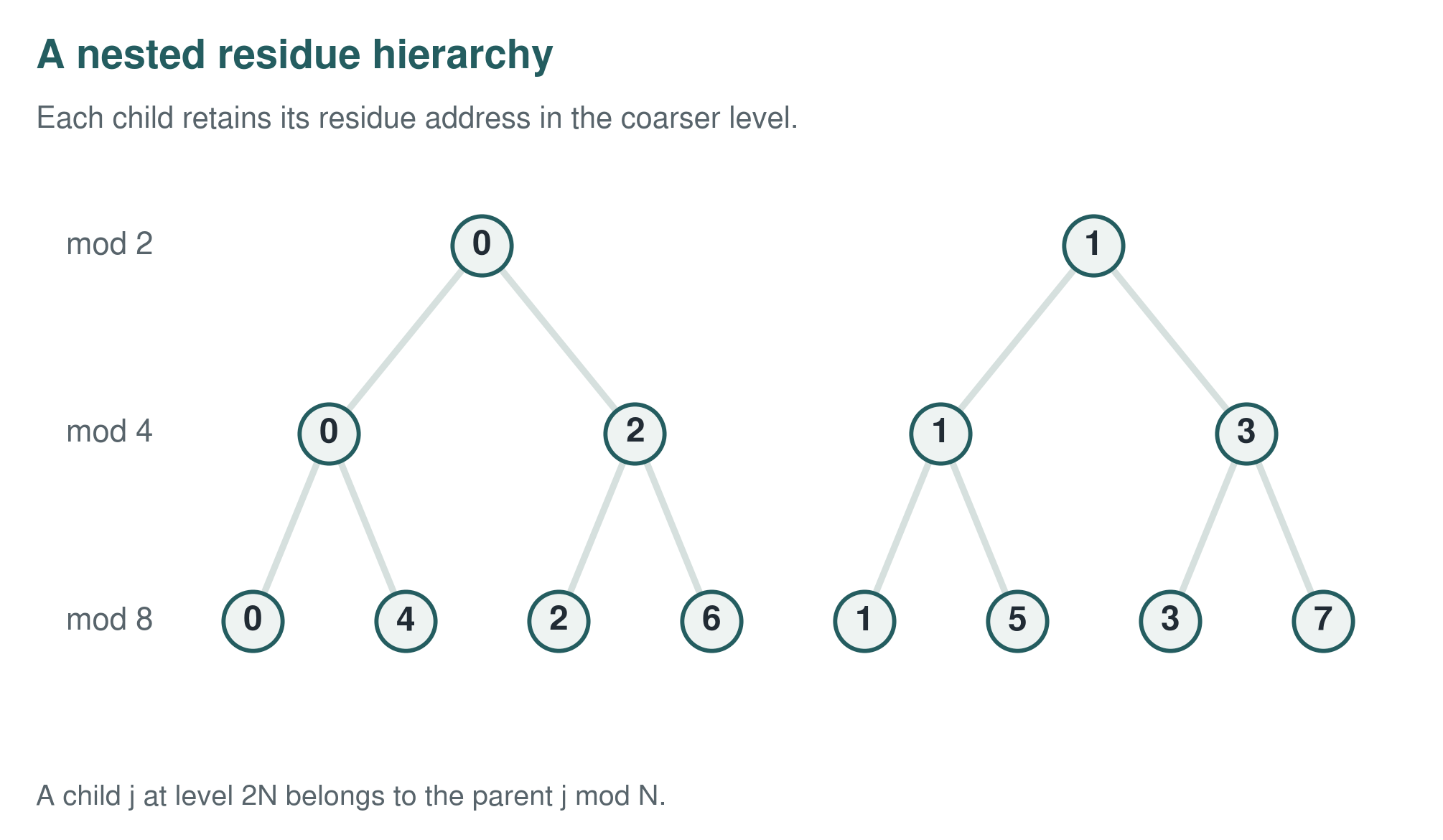
Theorem 4.6: Nested residue refinement

Let \(N,M\) be positive integers with \(N\) dividing \(M\), and let \(0\leq j<N\). Then

\[ P_{N,j} = \sum_{\substack{0\leq s<M\\s\equiv j\pmod N}}P_{M,s}. \]

When \(R\) is nonzero, the packet system modulo \(M\) refines the packet system modulo \(N\).

Read proof · Visual guide: Follow one coefficient through the tower · Read statement and proof side by side · Permalink · Source line 476 · Claim record · Lean coverage · Code · Worked examples

Proof of Theorem 4.6

An exponent \(n\) satisfies \(n\equiv j\pmod N\) exactly when its unique residue \(s\) modulo \(M\) satisfies \(s\equiv j\pmod N\).

Back to statement · Read statement and proof side by side · Permalink · Source line 486 · Claim record · Lean coverage · Code · Worked examples

Example 4.7: The shift graph of residue packets

Assume that \(R\) is nonzero and \(N>0\). Multiplication by \(z\) sends the residue packet \(P_{N,j}R[[z]]\) into \(P_{N,j+1}R[[z]]\), where the index is read modulo \(N\). Its packet graph is the directed cycle

\[ 0\longrightarrow1\longrightarrow\cdots\longrightarrow N-1\longrightarrow0. \]

Multiplication by a polynomial supported on a set of residues gives the corresponding finite set of phase shifts. This is the simplest transfer graph behind a polyphase representation.

Permalink · Source line 490

Theorem 4.8: Coprime factorization

Let \(A\) and \(B\) be coprime positive integers. For each \(j\) modulo \(AB\), write

\[ j_A=j\pmod A, \qquad j_B=j\pmod B. \]

Then

\[ P_{AB,j}=P_{A,j_A}P_{B,j_B}. \]

Every pair \((j_A,j_B)\) occurs for one residue \(j\) modulo \(AB\).

Read proof · Read statement and proof side by side · Permalink · Source line 498 · Claim record · Lean coverage · Code · Worked examples

Proof of Theorem 4.8

A coefficient survives the product on the right exactly when its exponent satisfies both congruences. The Chinese remainder theorem gives one residue class modulo \(AB\) with those two coordinates. The needed form of the theorem is standard and may be found in [Lang2002].

Back to statement · Read statement and proof side by side · Permalink · Source line 512 · Claim record · Lean coverage · Code · Worked examples

Corollary 4.9: Dyadic and odd coordinates

Write \(N=2^aM\) with \(M\) odd. Every residue packet modulo \(N\) is the product of one packet modulo \(2^a\) and one packet modulo \(M\).

Read proof · Visual guide: One address, two independent residues · Read statement and proof side by side · Permalink · Source line 516 · Claim record · Lean coverage · Code · Worked examples

Proof of Corollary 4.9

Apply Theorem 4.8 to the coprime moduli \(2^a\) and \(M\).

Back to statement · Read statement and proof side by side · Permalink · Source line 520 · Claim record · Lean coverage · Code · Worked examples

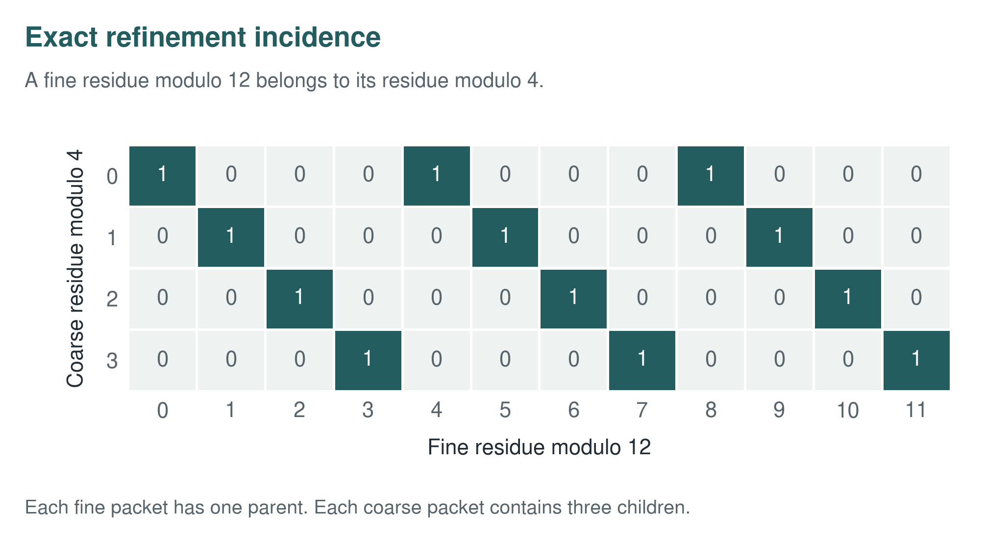
Example 4.10: Residues modulo twelve

The pair

\[ (j\pmod4,j\pmod3)=(3,1) \]

corresponds to \(j=7\) modulo \(12\). Hence

\[ P_{12,7}=P_{4,3}P_{3,1}. \]

This factorization concerns addresses. It does not say that the two factors have the same integral spectral behavior.

Permalink · Source line 524

A three-by-eight table gives every residue modulo 24 from its residue modulo three and residue modulo eight. — A composite residue packet is addressed by its dyadic and odd coordinates. The displayed mod-\(24\) system is the product of mod \(8\) and mod \(3\).

Source and conversion record

Source SHA-256: 810e4a615babb27fb5458b8252541e5f6069185221da02d31b71c3d319afa1ee

Unsupported prose commands stop the build. The mathematical expression sequence is checked against the source, with manuscript macros expanded for display.

Conversion records

Read and explore

Proofs and implementation

About this work

Other resources

3 Packet systems and refinement towers

Definition 3.1: Packet system

Definition 3.2: Refinement

Theorem 3.3: Children, parents, and transitivity

Proof of Theorem 3.3

Definition 3.4: Coordinate change across levels

The central idea

Theorem 3.5: Exact coordinate change and coherence

Proof of Theorem 3.5

Remark 3.6: Refinement and reduction

Corollary 3.7: Orthogonal Hilbert packets

Proof of Corollary 3.7

3.1 Typed coordinate naturality

How to read the result

3.2 Operator blocks across refinement

Theorem 3.8: Refinement of operator blocks

Proof of Theorem 3.8

Corollary 3.9: Support under refinement

Proof of Corollary 3.9

3.3 Common refinements

Theorem 3.10: Common refinement of commuting packet systems

Proof of Theorem 3.10

Proposition 3.11: Coarsest common refinement

Proof of Proposition 3.11

Example 3.12: A two level split

4 Residue coordinates and coprime factorization

Definition 4.1: Residue selector

Proposition 4.2: Residue packet algebra

Proof of Proposition 4.2

4.1 Finite orthogonality certificates

Theorem 4.3: Root-of-unity realization

Proof of Theorem 4.3

4.2 The field specialization

Theorem 4.4: Character realization

Proof of Theorem 4.4

Remark 4.5: Two distinct constructions

Theorem 4.6: Nested residue refinement

Proof of Theorem 4.6

Example 4.7: The shift graph of residue packets

Theorem 4.8: Coprime factorization

Proof of Theorem 4.8

Corollary 4.9: Dyadic and odd coordinates

Proof of Corollary 4.9

Example 4.10: Residues modulo twelve