
12 Worked realizations in the common operator language
On this page · Permalink · Source line 1
12.1 Signal polyphase coordinates
On this page · Permalink · Source line 3
Let \(x=(x_n)_{n\in{\mathbb Z}}\in c_{00}({\mathbb Z};R)\) and let the seed be \(\delta_0\) under the bilateral shifts \((S^r\delta_0)_n=\delta_{n,r}\). This makes the algebraic span and every displayed sum finite. The \(N\) packets are
Synthesis interleaves these sequences. A linear filter with a finite impulse response that is invariant under shifts becomes an \(N\times N\) matrix of transfer blocks. Refining from \(N\) to \(M\) with \(N\mid M\) splits each coarse phase into its descendants without changing the reconstructed signal. The same formulas extend to standard sequence completions when the synthesis series converges. This is the usual polyphase viewpoint from multirate filter banks [Vaidyanathan1993].
12.2 Sparsity of transfer blocks
On this page · Permalink · Source line 19
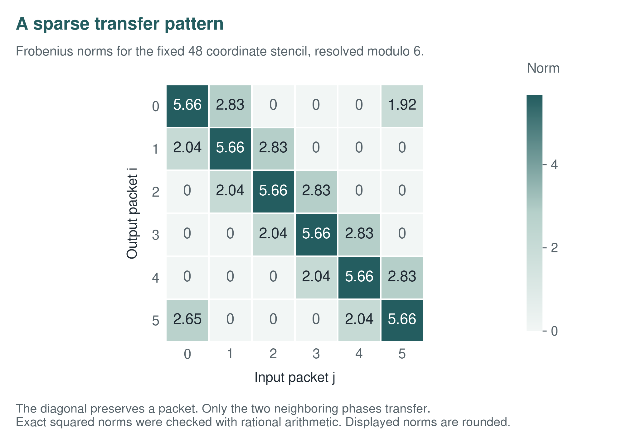
A banded operator need not remain banded after residue reordering, but its nonzero couplings become a structured packet graph. With the convention \((S_rx)_n=x_{n-r}\), the only active transfer is
with indices taken modulo \(N\). More general finite stencils produce a finite set of active phase differences.
12.3 A short realization in Smith chart coordinates
On this page · Visual guide: Two Smith constructions, different roles · Visual guide: Two Smith constructions, different roles · Permalink · Source line 36
How to read the result
The Smith chart used here is a coordinate diagram for impedance and reflection. It is different from the Smith normal form used earlier to study integral congruences. The connection within this paper is the way a change of coordinates makes an action easier to describe. Here a rotation in reflection coordinates becomes a fractional linear map in impedance coordinates. The sampled phase orbit is a geometric example and does not supply another linear projector decomposition.
Let \(Z\) and \(Z_0\ne0\) be complex impedances, put \(z=Z/Z_0\), and assume \(z\ne-1\). Write
On the open reflection disk \(|\Gamma|<1\), multiplication by any phase \(\omega_N^k\) stays in the disk and has a finite inverse-chart image. The phase action is
Outside the open disk, the same chart formula requires \(1-\omega_N^k\Gamma\ne0\). Pulling the phase action back on this domain gives
For \(N=2\) and \(k=1\),
Thus the nontrivial action at the first phase level exchanges normalized impedance and admittance. Calling these values “packets” is geometric terminology for the sampled orbit. It does not assert that the two values form linear idempotent ranges. Higher refinements at powers of \(2\) sample the same reflection circle at progressively finer electrical phases. Compare the standard Smith chart conventions in [pozar2012].

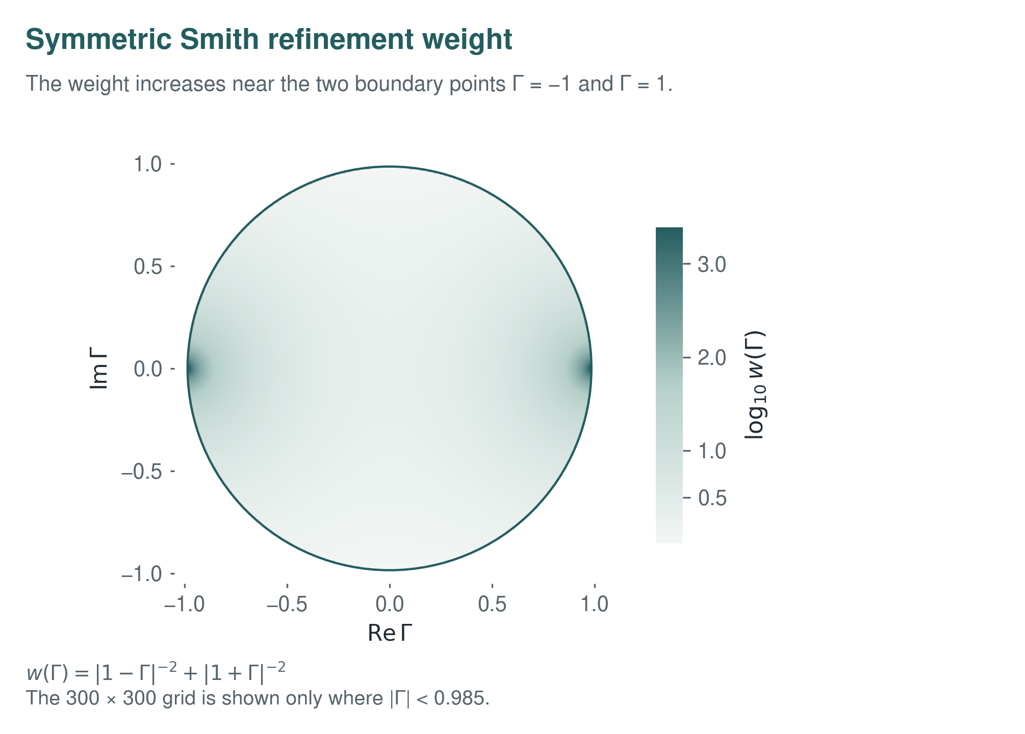
The symmetric weight
indicates where small errors in reflection coordinates produce large impedance or admittance errors.
13 Finite computational certificates
On this page · Permalink · Source line 96
The following results and tables are the recorded v1.2.1 finite implementation evidence. They do not certify the expanded lattice or analytic statements in Lean. Current reproduction outcomes are reported in the verification files accompanying this edition.
All numerical work in this paper is finite and reproducible. It tests the Python implementation of identities proved above or checked against certificates. It does not replace those arguments or the Lean kernel checks. Release 1.2.1 runs 48 tests, including contracts for invalid input, refinement transitivity, aggregation of transfer blocks, Fourier/DFT agreement, Smith fibre counts by exhaustive enumeration, and consistency of the stored JSON and CSV records.
| Check | Result |
|---|---|
| Packet synthesis residuals for moduli \(2,3,4,6,8,12\) | \(0\) |
| Nested refinement residuals for \(2\to4\), \(2\to8\), \(3\to6\), \(3\to12\), \(4\to8\), \(4\to12\), \(6\to12\) | \(0\) |
| CRT residuals for dyadic and odd moduli for \(4\times3\), \(8\times3\), \(4\times5\), \(8\times5\) | \(0\) |
| Maximum finite Fourier projector residual | \(6.60\times10^{-15}\) |
| Weighted inverse residual modulo \(2^{10}\) | \(0\) |
| Weighted inverse residual modulo \(3^8\) | \(0\) |
| Weighted inverse residual modulo \(5^7\) | \(0\) |
| Difference between filtered and direct modular inverses | \(0\) |
| Transfer zeta coefficients versus direct walk enumeration through weight \(30\) | exact match |
| Dyadic sign projector resultant weight | \(v_2(2)=1\) |
| Sign projector resultant weight at the odd prime \(3\) | \(v_3(2)=0\) |
| Power defect telescoping identity residual | at most \(6.94\times10^{-18}\) |
| Resolvent defect identity residual | \(1.09\times10^{-17}\) |
| Smith \(N=2\) phase versus \(z\mapsto1/z\) | residual below \(1.4\times10^{-16}\) |
Numerical certificate 13.1: Weighted inverse
For the tested diagonal-plus-transfer matrices, the filtered inverse agrees exactly with direct modular inversion at all tested precisions:
The maximum modular residual is zero in every case.
Permalink · Source line 133 · Claim record · Lean coverage · Code · Worked examples
Numerical certificate 13.2: Transfer zeta
The rational function
was expanded through degree \(30\). Every coefficient agrees with direct weighted-walk enumeration.
Permalink · Source line 141 · Claim record · Lean coverage · Code · Worked examples
Numerical certificate 13.3: Dyadic separation
The code verifies exactly that the two rational sign projectors are idempotent, orthogonal, and complementary, that scaling by \(2\) makes both integral, and that the same projectors are already integral modulo every tested odd prime.
Permalink · Source line 149 · Claim record · Lean coverage · Code · Worked examples
14 Scope and limits
On this page · Permalink · Source line 154
The exact statements above have several deliberate boundaries.
First, refinement changes coordinates while preserving reconstruction. If a numerical method discards fine packets, the resulting error must be estimated separately.
Second, the weighted inverse is linear. A nonlinear map creates higher order interactions among packet coordinates. Those interactions are not contained in the path formula of Theorem 5.2.
Third, a resultant is only a denominator bound. The exact weight depends on the lattice and is given by Theorem 8.2. The two examples in Example 7.4 and Example 8.10 show that the same eigenvalue separation can give different integral packet weights.
Fourth, the dyadic sign example is a model rather than a classification of all phenomena at the prime two. Character averages, trace splittings, quadratic refinements, and deformation projectors must each be checked on their own lattices.
Finally, the defect formulas do not prove that a chosen coarse operator is a good approximation. They say exactly how a known one step defect propagates. A useful approximation theorem must also bound that defect in the problem under study.
A Notation table
On this page · Permalink · Source line 171
| Symbol | Meaning |
|---|---|
| \(P_{\ell,\alpha}\) | packet projector at refinement level \(\ell\) |
| \(I_\ell\) | packet address set at level \(\ell\) |
| \(\beta\succ\alpha\) | fine packet \(\beta\) is a child of coarse packet \(\alpha\) |
| \({\mathcal A}_\ell,{\mathcal S}_\ell\) | packet analysis and synthesis maps |
| \(J_{\ell+1,\ell}\) | exact coordinate refinement map |
| \(C_{\ell,\ell+1}\) | exact coordinate regrouping from fine to coarse |
| \(T^{(\ell)}_{\beta\alpha}\) | transfer block \(P_{\ell,\beta}TP_{\ell,\alpha}\) |
| \(P_{N,j}\) | residue or phase selector for address \(j\pmod N\) |
| \(w(e)\) | positive filtration weight of a transfer edge |
| \(W(\gamma)\) | cumulative weight of a transfer word or graph walk |
| \(A(t)\) | polynomial weighted adjacency matrix |
| \(Z_{s,t}(t)\) | weighted transfer-zeta function from vertex \(s\) to vertex \(t\) |
| \(s_{\pi,\Lambda}(E)\) | separation weight of a rational projector on the chosen lattice, when a clearing exponent exists |
| \(\Delta\) | linear refinement defect for one step \(CT_f-T_cC\) |
B Algorithmic forms
On this page · Permalink · Source line 195
B.1 Residue analysis and synthesis
On this page · Visual guide: Filter first or split first: same output · Permalink · Source line 197
def analyze_residues(x, N):
    require N > 0
    return [x[j::N] for j in range(N)]

def synthesize_residues(packets):
    N = len(packets)
    require packet lengths fit one N-way interleaving
    y = empty(sum(len(p) for p in packets))
    for j, packet in enumerate(packets):
        y[j::N] = packet
return yThe verified contract is \(\operatorname{synthesize}(\operatorname{analyze}(x,N))=x\). The Lean counterpart uses packet coordinates restricted to projector ranges and proves both inverse laws. The finite Python routine checks the concrete array realization.
B.2 Weighted inverse at finite precision
On this page · Visual guide: The residual tells you when to stop · Permalink · Source line 219
Dinv = inverse(D)                       # certified on both sides
edge[e] = Dinv @ H_edge[e]
require Dinv @ H == sum(edge[e] for e in edges)
require edge[e] lies in filtration[weight[e]]
m = certified_lower_bound(weight)       # 1 <= m <= weight[e]
N = (L + m - 1) // m                    # so L <= m*N
S = 0
for n in range(N):
    for word in edge_tuples(edges, n):
        if sum(weight[e] for e in word) < L:
            S += (-1)**n * ordered_product(edge[e] for e in word)
return q_L(S @ Dinv)Lean proves that the mapped pruned sum is exactly the mapped finite geometric inverse. The lower bound \(m\) gives \(m|\gamma|\le W(\gamma)\), so \(L\le mN\) derives \(q_L(A^N)=0\) from the filtration certificate and makes the returned value an inverse on both sides of \(q_L(D+H)\). The Lean lemma \(L\le m\lceil L/m\rceil\) justifies the displayed executable cutoff for \(m>0\). Taking \(m=1\) and \(N=L\) gives the unconditional cutoff for positive weights. The Python implementation checks the DVR matrix specialization against direct modular inversion.
B.3 Walk construction for transfer zeta
On this page · Permalink · Source line 245
def coefficient(G, start, target, n):
    total = 0
    for length in range(n + 1):
        for word in edge_tuples(G, length):
            if is_walk(word, start, target) and weight(word) == n:
                total += 1
    return total

A[i,j] = sum(t**weight(e) for distinct edges e from i to j)
T = I - A
Q = det(T)
H = adjugate(T)
P = H[start, target]
assert Q.coeff(0) == 1
Z = coefficient_series(G, start, target)
prove Q * Z == PPositive weights make the coefficient loop finite because every contributing word has length at most \(n\). Lean proves the enumeration correct, derives its recurrence from the first edge, proves \((I-A)Z=I\), constructs the determinant/adjugate inverse, and identifies the two matrices by inverse uniqueness. Thus the normalized \(QZ=P\) identity and its induced recurrence follow from finite graph data. The Python companion repeats the exact symbolic construction as an executable check. The Lean proof does not use it as an oracle.
C Proof dependency map
On this page · Permalink · Source line 275
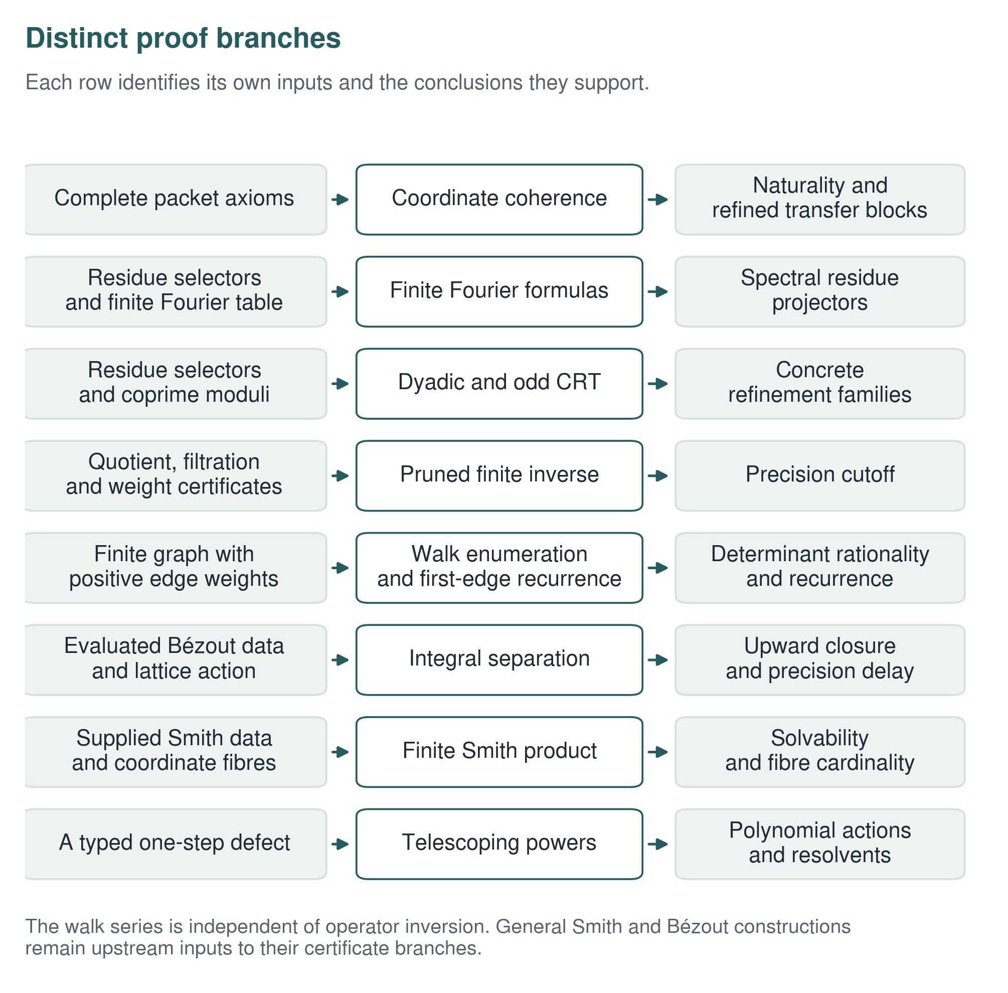
The proof order is:
The walk branch for transfer zeta is logically independent of operator inversion. Its rationality conclusion follows from finite graph data without a supplied \(QZ=P\) premise. Likewise, CRT factorization follows directly from residue selectors and coprimality. It does not require the abstract refinement theorem, although it supplies a concrete refinement family. General Smith diagonalization and the construction of polynomial Bézout/resultant data remain inputs to the formalized branches that use those certificates.