
5 Complete filtered transfer algebras
On this page · Permalink · Source line 1
A filtration records how deeply a term lies in the chosen notion of precision. The weights record guaranteed filtration gains that add under multiplication. A discrete valuation ring provides the main example.
Definition 5.1: Complete multiplicative filtration
A complete filtered algebra is a unital algebra \({\mathcal B}\) with a decreasing sequence of two-sided ideals
such that
and the natural map
is an isomorphism. A transfer term \(N_e\) has a declared positive integer weight \(w(e)\in\mathbb Z_{>0}\) when
Permalink · Source line 5 · Claim record · Lean coverage · Code · Worked examples
In the filtration topology, reduction to \({\mathcal B}/F^L{\mathcal B}\) is continuous when the quotient has the discrete topology. Its kernel \(F^L{\mathcal B}\) is therefore closed. In particular, a convergent sum of terms in \(F^L{\mathcal B}\) remains in that ideal.
If \({{\mathcal O}}\) is a complete discrete valuation ring with uniformizer \(\pi\) and \({\mathcal B}\) is a separated and complete \({{\mathcal O}}\) algebra for the filtration
then this is a standard example. Finite matrix algebras over \({{\mathcal O}}\) satisfy these conditions. Completeness of \({{\mathcal O}}\) alone does not imply completeness of every \({{\mathcal O}}\) algebra. Basic facts about completeness in this setting are reviewed in [Serre1979].
Theorem 5.2: Weighted inverse
Let \({\mathcal B}\) be a complete filtered algebra. Let \(D\in{\mathcal B}\) be invertible with
Let \(E\) be a finite set and suppose
Set
For a word \(\gamma=(e_1,\ldots,e_r)\), write
The empty word has weight zero and contributes the identity. Then \(T\) is invertible and
The series converges in the filtration, and the term indexed by \(\gamma\) belongs to \(F^{W(\gamma)}{\mathcal B}\).
Read proof · Read statement and proof side by side · Permalink · Source line 34 · Claim record · Lean coverage · Code · Worked examples
Proof of Theorem 5.2
Put
Since left multiplication by \(D^{-1}\) preserves the filtration, \(A\in F^1{\mathcal B}\). Completeness gives the convergent Neumann series
Because \(T=D(I+A)\),
Expanding each power of \(A\) gives the sum over words, with the rightmost edge acting first. Multiplicativity of the filtration gives
For each \(L\), only finitely many words have weight below \(L\) because \(E\) is finite and every edge has positive weight. Thus the word expansion converges to the same inverse.
Back to statement · Read statement and proof side by side · Permalink · Source line 66 · Claim record · Lean coverage · Code · Worked examples
The preceding formula does not yet use packet blocks. When \(D\) is packet diagonal and the terms \(N_e\) are individual transfers, only words with compatible packet endpoints can contribute. These words become directed paths.
Theorem 5.3: Block path formula
Let \({\mathcal P}=(P_\alpha)_{\alpha\in I}\) be a finite packet system in a complete filtered algebra of operators. Suppose
belongs to \({\mathcal B}\) and is invertible on every packet. Assume that the assembled inverse
where each packet inverse is extended by zero to the other packets. Let the edge set be finite, assume \(w(e)\geq1\) for every edge, and write
For an edge \(e:\alpha\to\beta\), put
Then the block from \(P_\alpha X\) to \(P_\beta X\) of \((D+N)^{-1}\) is
where \(D_\alpha=P_\alpha DP_\alpha\) and the sum runs over directed paths from \(\alpha\) to \(\beta\), including the empty path when \(\alpha=\beta\).
Read proof · Read statement and proof side by side · Permalink · Source line 88 · Claim record · Lean coverage · Code · Worked examples
Proof of Theorem 5.3
The diagonal inverse is
The block \(P_\beta D^{-1}NP_\alpha\) is nonzero only when there is a declared edge from \(\alpha\) to \(\beta\). Repeated block multiplication shows that the \(r\)th power of \(D^{-1}N\) is the sum over all directed paths of length \(r\), with the operator factors ordered along the path. Apply Theorem 5.2 and multiply on the right by the packet diagonal inverse.
Back to statement · Read statement and proof side by side · Permalink · Source line 120 · Claim record · Lean coverage · Code · Worked examples
Corollary 5.4: Minimum path weight
For packets \(\alpha\) and \(\beta\), let \(d(\alpha,\beta)\) be the least total weight of a directed path from \(\alpha\) to \(\beta\), with \(d=\infty\) when no path exists. Use the convention \(F^\infty{\mathcal B}=\bigcap_{L\geq0}F^L{\mathcal B}=0\). If \(\alpha\ne\beta\), then
If there is no path from \(\alpha\) to \(\beta\), the block is zero.
Read proof · Read statement and proof side by side · Permalink · Source line 128 · Claim record · Lean coverage · Code · Worked examples
Proof of Corollary 5.4
Every term in the block path formula is indexed by a path from \(\alpha\) to \(\beta\) and lies in the filtration level given by its total weight. If no such path exists, the sum is empty.
Back to statement · Read statement and proof side by side · Permalink · Source line 138 · Claim record · Lean coverage · Code · Worked examples
Example 5.5: A longer path that appears earlier
Consider three packets \(\alpha\), \(\beta\), and \(\gamma\). Suppose there is a direct edge from \(\alpha\) to \(\gamma\) of weight three, together with edges
of weight one each. The two edge route has total weight two, so it contributes to the inverse before the direct edge does. This is why the truncation rule uses total weight rather than path length. The lower bound in Corollary 5.4 need not be an equality because several paths of the same weight may cancel.
The central idea
Word length counts how many transfers are composed. Weight counts how much filtration gain those transfers guarantee. The sign in the inverse expansion depends on length, while the precision cutoff depends on weight. A short word can therefore disappear at a chosen precision while a longer word still contributes.
Corollary 5.6: Acyclic transfer graph
If the packet transfer graph is acyclic, then \(D^{-1}N\) is nilpotent. The inverse in Theorem 5.3 is a finite sum and does not require completeness of the filtration.
Read proof · Read statement and proof side by side · Permalink · Source line 156 · Claim record · Lean coverage · Code · Worked examples
Proof of Corollary 5.6
A finite acyclic directed graph has a bound on path length. Every sufficiently long product of transfer blocks is therefore zero. The Neumann series terminates.
Back to statement · Read statement and proof side by side · Permalink · Source line 160 · Claim record · Lean coverage · Code · Worked examples
Corollary 5.7: Stability of inversion at finite precision
Let \(T\) and \(\widetilde T\) be invertible elements of \(F^0{\mathcal B}\). If
then
Read proof · Read statement and proof side by side · Permalink · Source line 164 · Claim record · Lean coverage · Code · Worked examples
Proof of Corollary 5.7
Use the resolvent identity at zero in the form
Both inverse factors belong to \(F^0{\mathcal B}\), so the product lies in \(F^L{\mathcal B}\).
Back to statement · Read statement and proof side by side · Permalink · Source line 175 · Claim record · Lean coverage · Code · Worked examples
Corollary 5.8: Exact finite precision truncation
Under the hypotheses of Theorem 5.2, define
Then
Thus \(R_L\) is the exact inverse in \({\mathcal B}/F^L{\mathcal B}\).
Read proof · Read statement and proof side by side · Permalink · Source line 185 · Claim record · Lean coverage · Code · Worked examples
Proof of Corollary 5.8
Every omitted word has weight at least \(L\), so the difference from the full inverse lies in \(F^L{\mathcal B}\). Multiplication by \(T\) or by its inverse preserves membership in \(F^L{\mathcal B}\) under the stated filtration assumptions. The two residual statements follow.
Back to statement · Read statement and proof side by side · Permalink · Source line 204 · Claim record · Lean coverage · Code · Worked examples
Example 5.9: A triangular transfer
Let \({{\mathcal O}}\) be complete with uniformizer \(\pi\), and consider
with \(a\geq1\). The only nontrivial transfer has weight \(a\), and its square is zero. Hence
At precision \(L\leq a\), the transfer vanishes and the inverse is the identity modulo \(\pi^L\). At depth \(a+1\), the transfer between the two packets first becomes visible.
Two compatible word conventions.
On this page · Permalink · Source line 230
The path expansion above labels a word in chronological order and writes its operator product in reverse order, so the first edge acts first. The following finite-word contract uses written multiplication order. Reversing all word labels identifies the sums over all words. Individual path labels must retain their stated convention. The two conventions do not change a weight or an inverse.
5.1 Finite quotient and normed-ring realizations
On this page · Permalink · Source line 232
5.1.1 Normalized edges and written-word convention
On this page · Permalink · Source line 234
Let \({{\mathcal O}}\) be a complete discrete valuation ring with uniformizer \(\pi\), fraction field \(K\), and filtration
on an \({{\mathcal O}}\)-algebra \({\mathcal B}\). The finite quotient statements below do not require \({\mathcal B}\) itself to be complete. Suppose
where \(D\) is invertible and the perturbation \(H\) raises filtration. The symbol \(K\) is reserved for the fraction field.
A packet decomposition resolves \(H=\sum_{e\in E}H_e\) and assigns a certified filtration gain
Each \(e\) is a directed transfer edge. For an ordered transfer word
define
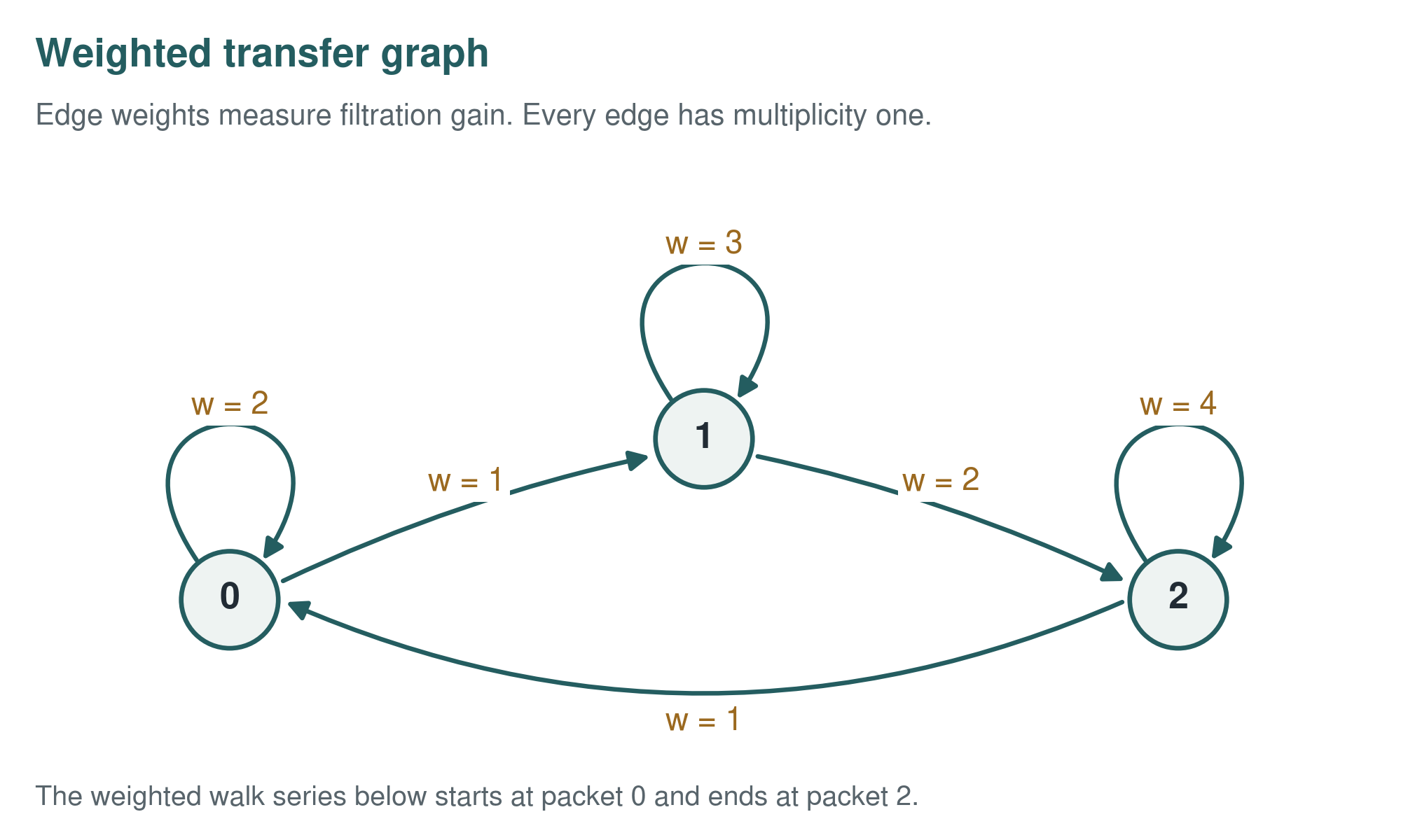
Theorem 5.10: Certified weighted inverse
Let \(R\) be a possibly noncommutative ring, let \(D^{-1}\) be a supplied two-sided inverse of \(D\), and put \(A=D^{-1}H\).
If \(A^r=0\), then \(D+H\) has the two-sided inverse
\[ \boxed{(D+H)^{-1}=\left(\sum_{k=0}^{r-1}(-A)^k\right)D^{-1}.} \]If \(R\) is a complete normed ring and \(\lVert A\rVert<1\), then \(\sum_{k\ge0}(-A)^k\) converges and
\[ \boxed{(D+H)^{-1}=\left(\sum_{k\ge0}(-A)^k\right)D^{-1}.} \]
Read proof · Visual guide: Three kinds of resolution · Visual guide: Which words can survive precision five? · Visual guide: An inverse computed in both orders · Visual guide: The residual tells you when to stop · Read statement and proof side by side · Permalink · Source line 273 · Claim record · Lean coverage · Code · Worked examples
Proof of Theorem 5.10
Factor
For a finite cutoff \(r\), multiplication on either side gives the noncommutative telescoping identity
This proves (a). In (b), the strict norm bound makes the geometric series summable. Continuity of multiplication passes the same identities to the limit. Multiplication by \(D^{-1}\) gives the displayed inverse in both orders.
Back to statement · Read statement and proof side by side · Permalink · Source line 289 · Claim record · Lean coverage · Code · Worked examples
Corollary 5.11: Finite precision
Let \(F^\bullet R\) be a multiplicative decreasing filtration and let \(q_L:R\to R_L\) be a ring homomorphism that kills \(F^L R\). Suppose
with \(E\) finite. Then \(q_L(D^{-1}H)^L=0\), the finite sum in Theorem 5.10(a) is a two-sided inverse after applying \(q_L\), and its word expansion may discard every word of weight at least \(L\). More explicitly, for a length cutoff \(N\), define
Lean proves directly that \(q_L(S^{\mathrm{pr}}_{L,N})\) equals the mapped geometric inverse whenever \(q_L(A^N)=0\), and hence is a two-sided inverse of \(q_L(I+A)\), where \(A=\sum_eA_e=D^{-1}H\). With the supplied two-sided inverse \(D^{-1}\) of \(D\), this gives the explicit two-sided inverse
If every edge weight is at least \(m\) and \(L\le mN\), then the nilpotence condition follows from the filtration data because \(m|\gamma|\le W(\gamma)\). For \(m>0\), the executable choice \(N=\lceil L/m\rceil\) satisfies \(L\le mN\). This elementary ceiling inequality is also proved in Lean. The choice \(m=1,N=L\) gives the standard cutoff. In the DVR example \(q_L:R\to R/\pi^L R\), this reads
Visual guide: Which words can survive precision five? · Visual guide: An inverse computed in both orders · Visual guide: The residual tells you when to stop · Permalink · Source line 309 · Claim record · Lean coverage · Code · Worked examples
Here \(A_\gamma=(D^{-1}H_{e_1})\cdots(D^{-1}H_{e_r})\) in the written order. Multiplicativity places it in \(F^{W(\gamma)}R\), so the quotient kills it when \(W(\gamma)\ge L\). Positive weights also imply \(|\gamma|\le W(\gamma)\), making the retained search finite.
How to read the result
Using the standard length cutoff, every discarded word has weight at least the chosen depth and vanishes in the quotient. The retained sum therefore satisfies both inverse identities exactly at that precision. The earlier truncation theorem states the corresponding residual bounds in the complete filtered algebra itself.
The inherited finite-word contract proves the result in the finite quotients above and in the contraction specialization for complete normed rings. The complete filtered statement has its own separation and inverse-limit completeness hypotheses. Its current Lean coverage is recorded separately in the current correspondence.

6 Rational weighted transfer series
On this page · Permalink · Source line 368
A finite weighted graph records which path terms can occur in the inverse. Collecting paths by total weight turns this support information into a generating function. The finite adjacency matrix makes that function rational.
Definition 6.1: Weighted transfer series
Let \(G\) be a finite directed multigraph. Give every edge \(e\) a positive integer weight \(w(e)\) and a scalar multiplicity \(m(e)\) in a field \({\Bbbk}\). Define the polynomial adjacency matrix
For column vectors \(u\) and \(v\), define
where
Here \(\gamma=(e_1,\ldots,e_{|\gamma|})\) is a directed walk. Vertices and edges may repeat, and the empty walk has weight zero and multiplicity one. Thus the endpoint vectors weight the start and end of each walk, rather than only selecting subsets of vertices.
Permalink · Source line 372 · Claim record · Lean coverage · Code · Worked examples
Theorem 6.2: Rationality of the transfer series
The weighted transfer series satisfies
It is a rational function whose denominator divides
Read proof · Read statement and proof side by side · Permalink · Source line 393 · Claim record · Lean coverage · Code · Worked examples
Proof of Theorem 6.2
Since every entry of \(A(t)\) has zero constant term, the inverse exists in the formal power series ring and
The \((i,j)\) entry of \(A(t)^r\) is the sum of the monomials attached to all paths of length \(r\) from \(i\) to \(j\). Summing over \(r\) records paths of every length. Multiplication by the endpoint vectors gives the stated series. The adjugate formula gives
so every entry is rational.
Back to statement · Read statement and proof side by side · Permalink · Source line 406 · Claim record · Lean coverage · Code · Worked examples
Corollary 6.3: Recurrence for path counts
Write
Use the convention \(\deg 0=-\infty\). Then, for every nonnegative integer \(n>\deg P\),
Read proof · Read statement and proof side by side · Permalink · Source line 420 · Claim record · Lean coverage · Code · Worked examples
Proof of Corollary 6.3
Compare coefficients in the identity
Beyond the degree of \(P\), the coefficient on the right is zero.
Back to statement · Read statement and proof side by side · Permalink · Source line 433 · Claim record · Lean coverage · Code · Worked examples
In the recurrence, set \(a_k=0\) when \(k<0\). This is the coefficient convention for the formal power series \(Z_{u,v}(t)\) and makes the first recurrence equations meaningful even when \(n<d\).
Corollary 6.4: Several independent weights
Suppose every edge has a weight vector
Replace \(t^{w(e)}\) by
The resulting multigraded transfer series is rational in \(t_1,\ldots,t_r\).
Read proof · Read statement and proof side by side · Permalink · Source line 443 · Claim record · Lean coverage · Code · Worked examples
Proof of Corollary 6.4
The same matrix inverse proof works over the formal power series ring in several variables. The adjugate formula gives rationality.
Back to statement · Read statement and proof side by side · Permalink · Source line 455 · Claim record · Lean coverage · Code · Worked examples
The multigraded form is useful when dyadic depth, odd depth, and another filtration are tracked separately rather than collapsed into one number.
Example 6.5: A transfer series with one loop
Take vertices \(0\), \(1\), and \(2\). Give the edge \(0\to1\) weight one, the loop \(1\to1\) weight two, and the edge \(1\to2\) weight one. Every path from \(0\) to \(2\) uses the first and last edges and may traverse the loop any number of times. Hence
There is one path at every positive even weight and no path at an odd weight. The denominator records the increase of two units produced by the loop.
6.1 Automatic finite-graph construction
On this page · Permalink · Source line 473
Let \(G\) be a finite directed graph with positive integer edge weights. Define the polynomial adjacency matrix
where parallel edges are distinct elements of the finite edge type and are therefore counted with their full multiplicity.
For fixed start and target vertices \(s,t\), define
where \(a_n(s,t)\) counts directed walks from \(s\) to \(t\) with total weight \(n\). Vertices and edges may repeat. Thus “path zeta” is retained as the name of the series and Lean API, but the walks are not required to visit each vertex only once.
Theorem 6.6: Automatic finite-graph transfer-zeta rationality
Assume the vertex and edge sets are finite and every edge has positive integer weight. For every \(n\), exact enumeration of edge tuples of lengths at most \(n\), followed by endpoint and total-weight filtering, returns \(a_n(s,t)\). These coefficients obey the recurrence obtained by removing the first edge
Let
Then \(Q(0)=1\), hence \(Q\ne0\) and \(Q\) is a unit in \({\mathbb Z}[[t]]\), and the independently enumerated walk series satisfies
Read proof · Visual guide: Walks are not simple paths · Visual guide: A finite graph produces its denominator · Read statement and proof side by side · Permalink · Source line 494 · Claim record · Lean coverage · Code · Worked examples
Proof of Theorem 6.6
Every edge has weight at least one, so a word of weight \(n\) has length at most \(n\). The enumerator therefore searches a finite set containing every contributing walk, and its filters are exactly the defining predicates for \(a_n\). Removing the first edge gives the displayed disjoint decomposition into the empty diagonal walk and the first-edge tails. In matrix form this is
Positive weights give \(A(0)=0\), so \(T(0)=I\) and \(Q(0)=\det(I)=1\). The two adjugate identities
remain valid after inclusion into \({\mathbb Z}[[t]]\). Multiplying the adjugate by the formal-series inverse of \(Q\) constructs a two-sided inverse of \(T\). Uniqueness of the inverse identifies that construction with the independently enumerated matrix \(Z\), yielding the entrywise formulas.
Back to statement · Read statement and proof side by side · Permalink · Source line 524 · Claim record · Lean coverage · Code · Worked examples
This is the finite transfer-matrix method of [Stanley2012], but here its determinant, adjugate, normalization, recurrence from the first edge, and identification with the enumerated series are all formalized. The older API accepting an independently supplied normalized coefficient identity \(QZ=P\) is retained for external certificates. It is no longer needed to obtain rationality for the finite graph defined above. The Python companion performs an exact symbolic construction as an independent executable check.
Corollary 6.7: Linear recurrence
With the canonical polynomials from Theorem 6.6, write
Then the walk counts satisfy the recurrence with constant coefficients determined by \(Q\) after the finite initial range contributed by \(P_{s,t}\), with \(\deg 0=-\infty\):
Visual guide: A finite graph produces its denominator · Permalink · Source line 555 · Claim record · Lean coverage · Code · Worked examples
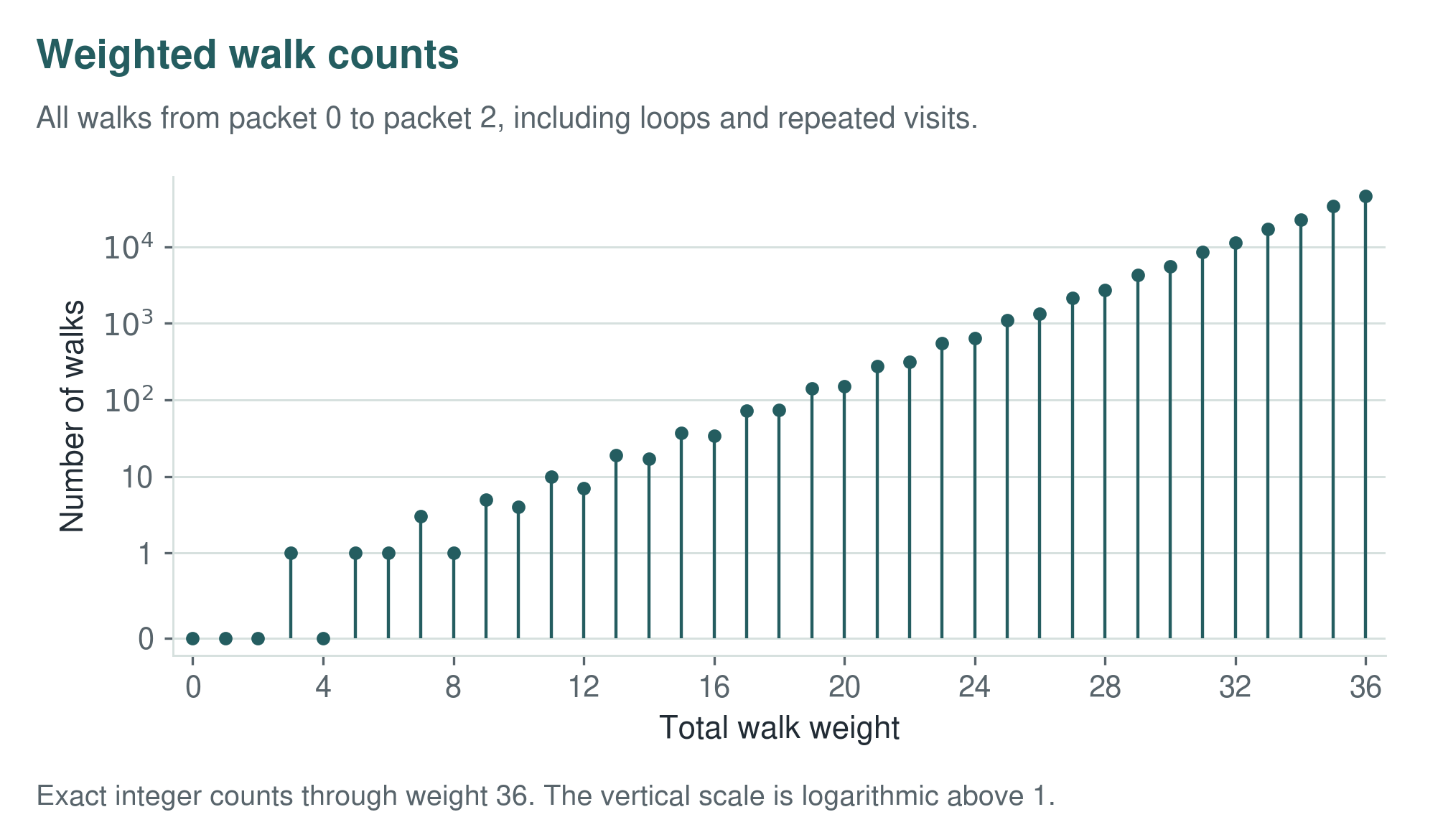
Example 6.8: A computed transfer zeta
For the graph used in the numerical companion, the walk series from packet \(0\) to packet \(2\) is
The first nonzero coefficients are
at their corresponding weights. Direct enumeration through weight \(30\) agrees coefficient by coefficient with the rational expansion.