
11 Linear refinement defects
On this page · Permalink · Source line 1
Exact coordinate refinement describes two representations of the same object. In an application, the coarse operator may instead be chosen to model coarse dynamics. An intertwining defect measures the mismatch between applying the operator before or after passing to coarse coordinates.
Let \(X_f\) and \(X_c\) be vector spaces or Banach spaces over a common field, and let
be a linear map, and let
Define
The central idea
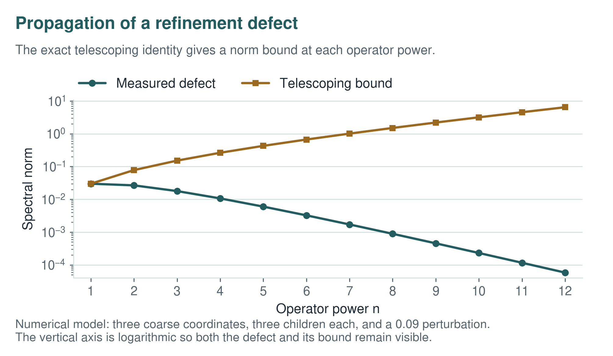
There are two routes from a fine state to a coarse result. One applies the fine operator and then maps the result to the coarse space. The other maps the state first and then applies the coarse operator. The defect is the difference between these routes. Its vanishing says that the chosen operators are compatible with the comparison map. The norm estimates below combine the size of this defect with the norms of the surrounding operators.
Theorem 11.1: Power defect identity
For every integer \(n\geq1\),
Read proof · Visual guide: A small defect can grow under powers · Read statement and proof side by side · Permalink · Source line 25 · Claim record · Lean coverage · Code · Worked examples
Proof of Theorem 11.1
The statement is clear for \(n=1\). For the induction step, write
and apply the induction hypothesis.
Back to statement · Read statement and proof side by side · Permalink · Source line 34 · Claim record · Lean coverage · Code · Worked examples
Corollary 11.2: Power norm bound
For bounded operators between Banach spaces,
Read proof · Read statement and proof side by side · Permalink · Source line 44 · Claim record · Lean coverage · Code · Worked examples
Proof of Corollary 11.2
Apply the triangle inequality and submultiplicativity to Theorem 11.1.
Back to statement · Read statement and proof side by side · Permalink · Source line 55 · Claim record · Lean coverage · Code · Worked examples
Corollary 11.3: Norm bound
For a submultiplicative operator norm,
If \(\|T_f\|,\|T_c\|\le\rho\), then
Visual guide: A small defect can grow under powers · Permalink · Source line 60 · Claim record · Lean coverage · Code · Worked examples
Corollary 11.4: Polynomial defect
For
we have
Read proof · Read statement and proof side by side · Permalink · Source line 78 · Claim record · Lean coverage · Code · Worked examples
Proof of Corollary 11.4
The constant terms cancel because \(CI=IC\). Apply Theorem 11.1 to every positive power and sum.
Back to statement · Read statement and proof side by side · Permalink · Source line 92 · Claim record · Lean coverage · Code · Worked examples
Theorem 11.5: Resolvent defect identity
If \(z-T_f\) and \(z-T_c\) are invertible, then
Read proof · Visual guide: Resolvents amplify errors near poles · Read statement and proof side by side · Permalink · Source line 96 · Claim record · Lean coverage · Code · Worked examples
Proof of Theorem 11.5
Multiply the claimed identity on the left by \(z-T_c\) and on the right by \(z-T_f\). The left side becomes
Multiplying back by the two resolvents proves the formula.
Back to statement · Read statement and proof side by side · Permalink · Source line 105 · Claim record · Lean coverage · Code · Worked examples
11.1 Inverse witnesses from one side and norm control
On this page · Permalink · Source line 117
For continuous linear maps, the same identity gives the certified norm bound
from a left inverse witness for the coarse scalar shift and a right inverse witness for the fine scalar shift. These witnesses suffice for the displayed identity. On their own, they need not define inverses on both sides and hence need not define resolvents. If \(\Delta=0\), Lean also proves, for every finite polynomial \(p\), the exact compatibility
in both the algebraic setting and the setting of continuous linear maps. Thus all powers and polynomial actions intertwine with coarse reconstruction. The stated inverse witnesses also intertwine. In particular, genuine resolvents do so when the scalar shifts are invertible. This is the linear prototype of the more general theory of refinement defects reserved for Paper III.
11.2 Analytic functional calculus
On this page · Permalink · Source line 147
Theorem 11.6: Holomorphic functional calculus defect
Let \(X_f\) and \(X_c\) be complex Banach spaces, and let \(C:X_f\to X_c\), \(T_f\), and \(T_c\) be bounded complex-linear maps. Let \(h\) be holomorphic on an open set \(U\) containing both spectra. Let \(\Gamma\) be an admissible finite rectifiable Cauchy cycle in \(U\) and in both resolvent sets, with winding number one on the union of the spectra and zero outside \(U\). The length of a cycle counts multiplicities. Then
Consequently,
Read proof · Read statement and proof side by side · Permalink · Source line 148 · Claim record · Lean coverage · Code · Worked examples
Proof of Theorem 11.6
The assertion is immediate if either space is zero. Otherwise, use the rectifiable-cycle form of the holomorphic functional calculus in [Conway1990], Chapter VII, §4, Theorem 4.1, formula (4.5), and Proposition 4.6. For each operator \(T\), compare \(\Gamma\) with a positive simple system around its spectrum. Their difference has zero winding outside \(U\setminus\sigma(T)\), so Theorem 4.1 applied to the resolvent-valued integrand identifies the two integrals. Consequently,
Subtract the two formulas after composing with \(C\), then use Theorem 11.5 inside the integral. The norm estimate follows from the standard contour bound.
Back to statement · Read statement and proof side by side · Permalink · Source line 169 · Claim record · Lean coverage · Code · Worked examples
Theorem 11.7: Exponential defect identity
Let \(C:X_f\to X_c\), \(T_f\), and \(T_c\) be bounded linear maps between Banach spaces over a common field. For real \(t\), use real or complex spaces. For complex \(t\), use complex spaces and complex-linear maps. Then
where the integral is taken along the straight segment from \(0\) to \(t\) when \(t\) is complex. For real \(t\geq0\),
Read proof · Read statement and proof side by side · Permalink · Source line 180 · Claim record · Lean coverage · Code · Worked examples
Proof of Theorem 11.7
For real \(t\), differentiate
We obtain
Integration from \(0\) to \(t\) gives the identity. The complex statement follows by the same calculation along the straight segment. The norm bound follows from the integral formula.
Back to statement · Read statement and proof side by side · Permalink · Source line 198 · Claim record · Lean coverage · Code · Worked examples
11.3 Several refinement levels
On this page · Permalink · Source line 210
Let
be linear maps for \(0\leq\ell<L\), and let \(T_\ell\in{\operatorname{End}}(X_\ell)\). Put
For \(a<b\), write
with \(C_{a,a}=I\).
Theorem 11.8: Multilevel defect decomposition
The total defect from level \(L\) to level zero is
For bounded maps,
Read proof · Read statement and proof side by side · Permalink · Source line 226 · Claim record · Lean coverage · Code · Worked examples
Proof of Theorem 11.8
Insert the intermediate terms
for \(0\leq\ell\leq L\). Consecutive differences telescope. The difference between the terms indexed by \(\ell+1\) and \(\ell\) is
Summing gives the identity. The norm estimate follows from the triangle inequality.
Back to statement · Read statement and proof side by side · Permalink · Source line 245 · Claim record · Lean coverage · Code · Worked examples
How to read the result
The multilevel formula keeps track of where each mismatch enters. A defect at one level is composed with the comparison maps needed to reach the input and output levels. The norm estimate therefore depends on both the local defects and the maps that carry them through the hierarchy. Controlling local mismatches alone does not control the total error if those maps amplify them.
Example 11.9: A visible one step defect
Let \(X_f={\Bbbk}^2\), let \(X_c={\Bbbk}\), and let
Take
Then
The coarse operator is exactly compatible with the fine operator precisely when the discarded coordinate does not feed into the retained coordinate. The entry \(c\) does not appear in the one step defect because it moves information in the opposite direction. It can still affect later powers through the terms in Theorem 11.1.
Corollary 11.10: Exact compatibility
If every one step defect \(\Delta_\ell\) vanishes, then
for every polynomial \(p\). The analogous resolvent, holomorphic, and exponential identities also hold whenever the relevant expressions are defined.
Read proof · Read statement and proof side by side · Permalink · Source line 283 · Claim record · Lean coverage · Code · Worked examples
Proof of Corollary 11.10
The total one step defect vanishes by Theorem 11.8. Apply Corollary 11.4, Theorem 11.5, Theorem 11.6, and Theorem 11.7.
Back to statement · Read statement and proof side by side · Permalink · Source line 291 · Claim record · Lean coverage · Code · Worked examples