Special FunctionsReading edition

The resolution atlas

Reading tools
Reading libraryInspect Lean
Switch work

Saved reading

Read side by side

Start reading

Resources & source

Read and explore

Proofs and implementation

About this work

Other resources

Original TeX with line links

Skip contents and start reading

A small change can alter the global order

A feedback channel may be almost invisible on a fixed disk and still determine the eventual growth of the function. Consider the normalized entire solution

\[ F_\varepsilon'(z)=1+(1-\varepsilon)F_\varepsilon(z/4)^2 +\varepsilon F_\varepsilon(3z/4)^2, \qquad F_\varepsilon(0)=0. \]

Here \(0\le\varepsilon\le1\). At \(\varepsilon=0\), its entire order is \(1/2\). At every positive weight, the order becomes \(\rho=\log2/\log(4/3)\approx2.40942084\).
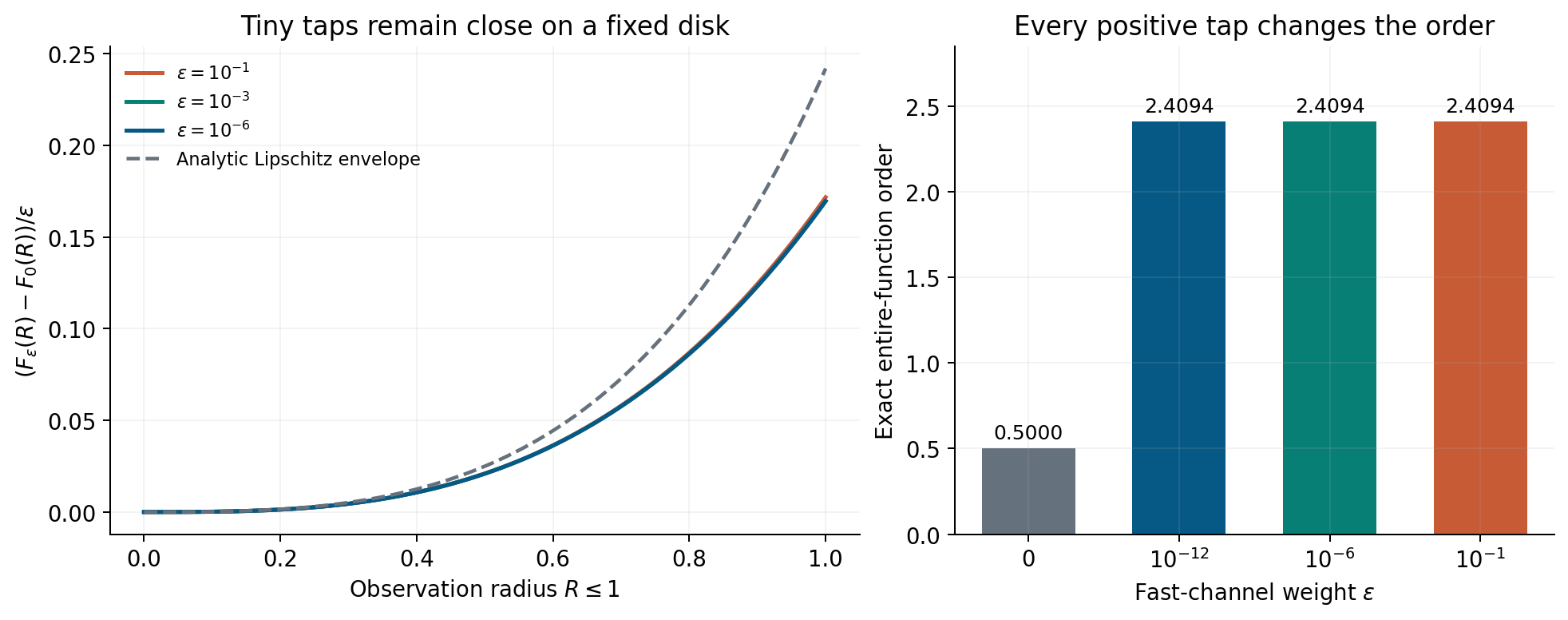
Left: divide the compact difference by the tap weight to compare its shape. Right: the proved order jumps at zero. The dashed curve is an analytic envelope. The function curves use 100-digit arithmetic and have a normalized omitted-series bound below 5.26 times 10 -23 on 0 less than or equal R less than or equal 1. Floating rounding is separate from that tail bound.
Left: divide the compact difference by the tap weight to compare its shape. Right: the proved order jumps at zero. The dashed curve is an analytic envelope. The function curves use 100-digit arithmetic and have a normalized omitted-series bound below \(5.26\times10^{-23}\) on \(0\le R\le1\). Floating rounding is separate from that tail bound.

View full-size figure (new tab)

The unit disk comes with an exact error certificate

Let \(f_{3/4}=F_1\), with \(f_{3/4}(z)=\sum_{n\ge0}d_nz^{2n+1}\). Positive coefficients give

\[ \sup_{|z|\le R}|F_\varepsilon(z)-F_0(z)| \le\varepsilon\sum_{n\ge1}nd_nR^{2n+1}. \]

A rational coefficient sum and a positive-tail estimate prove that, on the unit disk, the multiplier is less than \(0.241890267\). For \(\varepsilon=10^{-12}\), the entire disk therefore changes by less than \(2.41890267\times10^{-13}\).

The observation window and the global invariant answer different questions. Exact measurements can distinguish the functions. With an absolute error allowance at least half the displayed bound, midpoint data can fit both. The order concerns the limit through arbitrarily large radii, where the active faster channel eventually matters.

How far is far enough to guarantee separation?

The growth theorem supplies positive lower type for the weak-tap function and finite upper type for the slow function. For \(0<\varepsilon\le1\) and \(R\ge e\),
\[ \log F_\varepsilon(R)\ge c_\varepsilon R^\rho, \qquad \log F_0(R)\le C_0\sqrt R, \]
\[ c_\varepsilon=\frac{\log2}{(4/\varepsilon+8/3)^\rho}, \qquad C_0=e^{-1/2}(1+22\log2). \]
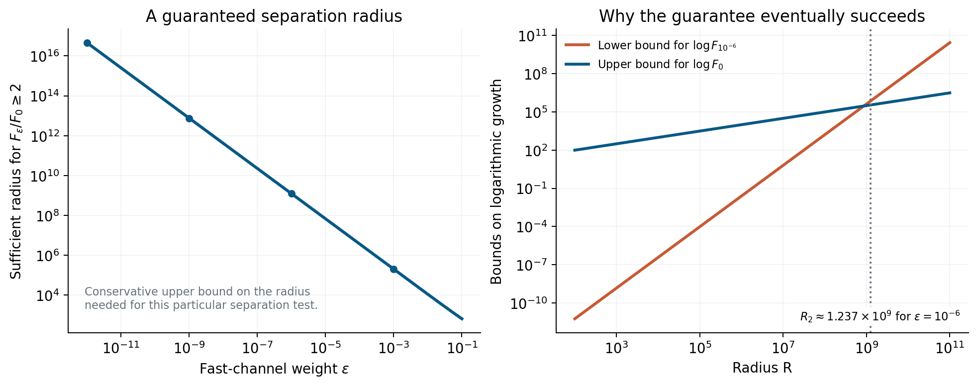
The left curve is a sufficient radius obtained from conservative comparison constants. The right panel shows why the lower bound for the perturbed function eventually exceeds the upper bound for the slow one. These are bounds on logarithmic growth, rather than numerical evaluations at the large plotted radii.

View full-size figure (new tab)

An explicit sufficient radius

Put

\[ R_2(\varepsilon)=\max\!\left\{ e,\left(\frac{2C_0}{c_\varepsilon}\right)^{1/(\rho-1/2)}, \left(\frac{2\log2}{c_\varepsilon}\right)^{1/\rho}\right\}. \]

Then \(F_\varepsilon(R)\ge2F_0(R)\) for every \(R\ge R_2(\varepsilon)\). The formula makes \(c_\varepsilon R^\rho\) at least both \(2C_0\sqrt R\) and \(2\log2\), and therefore at least their half-sum. Exponentiating gives the factor of two.

For \(\varepsilon=10^{-6}\), the formula is approximately \(1.237\times10^9\). This large radius is a guaranteed sufficient choice. It is not the first radius at which a useful difference appears, and it does not establish failure of every observation at smaller radii. The exact formula carries the guarantee. Rounded figures illustrate its scale.

A large excluded prime hides in a fixed window

Use the squarefree arithmetic family

\[ A_Q(s)=\sum_{\substack{n\ge2\\\mu(n)^2=1\\(n,Q)=1}} n^{-4}(1-n^{-2})^{2s}, \qquad D_p(s)=A_1(s)-A_p(s), \]

where \(p\) is prime. The difference contains exactly the squarefree atoms divisible by \(p\). Its largest frequency is \(\lambda_p=-2\log(1-p^{-2})\), and its total mass is \(D(4)/(p^4+1)\), with \(D(4)=105/\pi^4\).
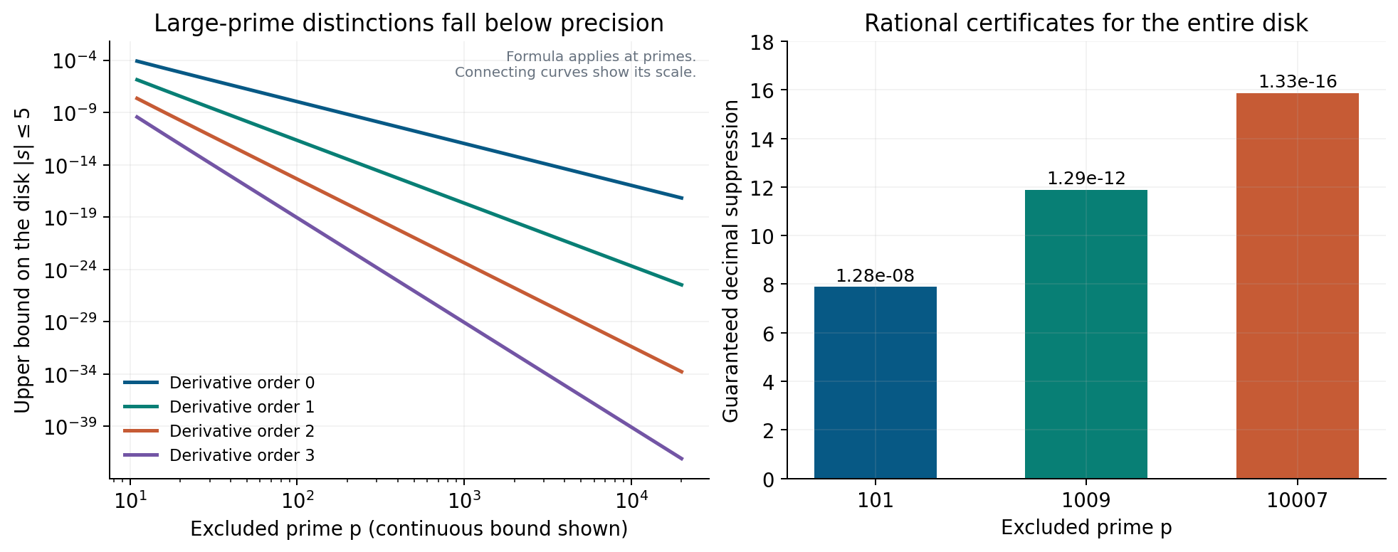
Left: analytic bounds for the function and three derivatives on |s| less than or equal 5. The connecting curves show scale, while the arithmetic statement applies at primes. Right: rational bounds for three particular excluded primes. The bar height is the negative base-ten logarithm of the bound, not a count of recovered digits.
Left: analytic bounds for the function and three derivatives on \(|s|\le5\). The connecting curves show scale, while the arithmetic statement applies at primes. Right: rational bounds for three particular excluded primes. The bar height is the negative base-ten logarithm of the bound, not a count of recovered digits.

View full-size figure (new tab)

The full complex disk has a rational certificate

For integer \(k\ge0\),

\[ \sup_{|s|\le5}|D_p^{(k)}(s)| <\frac{4(1-p^{-2})^{-10}}{3(p^4+1)} \left(\frac{2}{p^2-1}\right)^k. \]

The inequality uses \(D(4)<4/3\) and \(\lambda_p\le2/(p^2-1)\). Every quantity on the right is rational. For \(k=0\), upward decimal bounds are \(1.283\times10^{-8}\) at \(p=101\), \(1.287\times10^{-12}\) at \(p=1009\), and \(1.330\times10^{-16}\) at \(p=10007\).

The excluded prime changes the exact inverse of the function. Nevertheless, its effect becomes arbitrarily small on every fixed disk, including in every fixed derivative order. A bounded error model therefore needs an arithmetic parameter bound if it is to promise uniform recovery.

Seeing the prime can make subtraction harder

At negative real depth, the difference grows. The prime atom alone supplies a lower bound, while the entire removed shelf supplies an upper bound:

\[ p^{-4}e^{\lambda_pT}\le D_p(-T) \le\frac{D(4)}{p^4+1}e^{\lambda_pT},\qquad T\ge0. \]

Choose a tolerance \(\eta>D(4)/(p^4+1)\). Its unique crossing occurs between
\[ T_- =\frac{\log\!\bigl(\eta(p^4+1)/D(4)\bigr)}{\lambda_p}, \qquad T_+ =\frac{\log(\eta p^4)}{\lambda_p}. \]
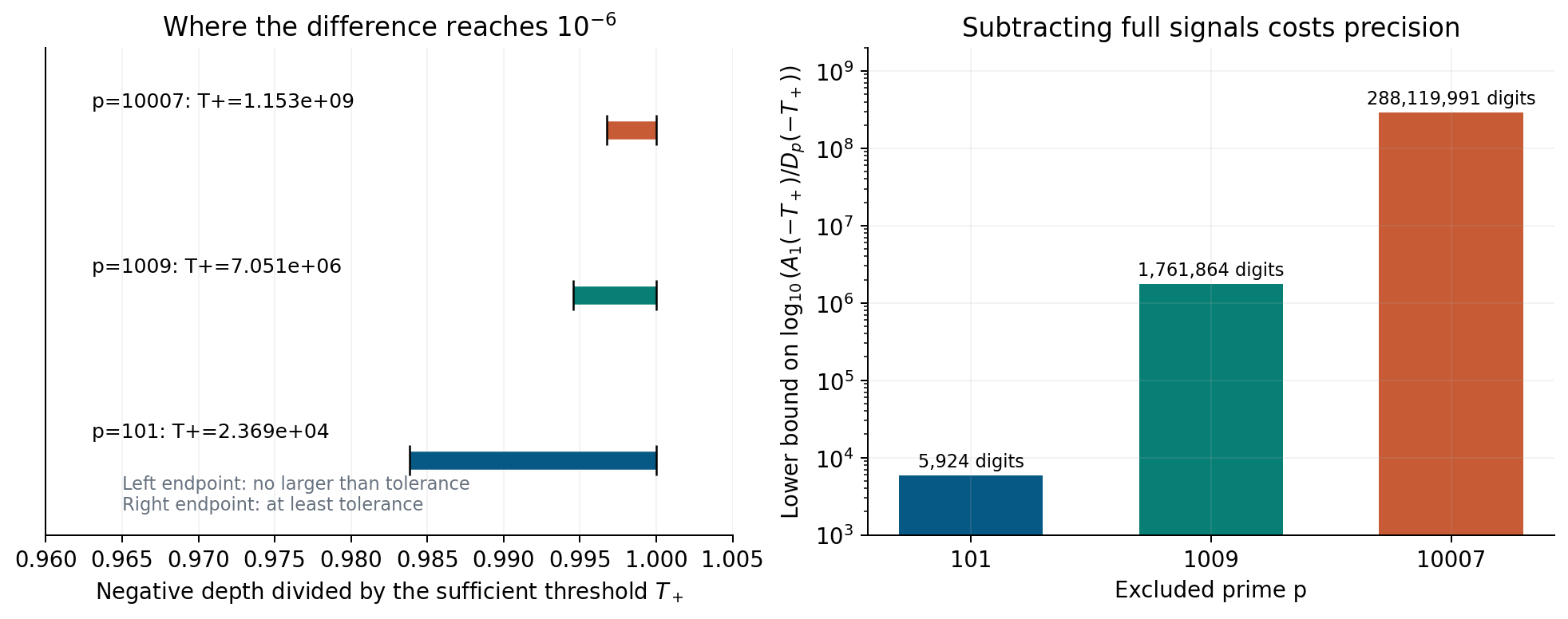
At tolerance 10 -6 , the left panel shows the analytic crossing brackets after rescaling each row by T +. The right panel shows a lower bound on the decimal cancellation scale when subtracting full functions. Displayed endpoints and labels are ordinary floating evaluations of exact formulas.
At tolerance \(10^{-6}\), the left panel shows the analytic crossing brackets after rescaling each row by \(T_+\). The right panel shows a lower bound on the decimal cancellation scale when subtracting full functions. Displayed endpoints and labels are ordinary floating evaluations of exact formulas.

View full-size figure (new tab)

For \(p=101\), the difference is no larger than \(10^{-6}\) through \(T_-=23307.789\ldots\), and at least that large by \(T_+=23690.516\ldots\). The decimals illustrate the formulas and are not rounded interval certificates.

The direct positive difference and subtraction have different costs

The \(n=2\) atom in the full function proves

\[ \frac{A_1(-T)}{D_p(-T)} \ge\frac{p^4+1}{16D(4)}e^{(\lambda_2-\lambda_p)T}. \]

At \(T_+\) for \(p=101\), the base-ten logarithm of this lower bound is about 5924. Subtracting independently approximated full functions can therefore amplify relative errors enormously. Evaluating the known positive difference series is a different procedure. These conditioning figures impose no universal precision requirement on every possible recovery algorithm.

A degree-seven witness exposes a signed defect

Let \(x_n=(1-n^{-2})^2\), and change the prime-two sieve strength to \(\lambda_2=-1-\delta\). For a real polynomial \(f\), the associated quadratic form is

\[ Q_\delta(f)=\sum_{\substack{n\ge1\\\mu(n)^2=1\\n\text{ odd}}} \frac{f(x_n)^2}{n^4} -\delta\sum_{\substack{n\ge1\\\mu(n)^2=1\\n\text{ even}}} \frac{f(x_n)^2}{n^4}. \]

Every even squarefree atom has negative mass. At \(\delta=10^{-12}\), the polynomial below certifies that this is detectable at finite degree.
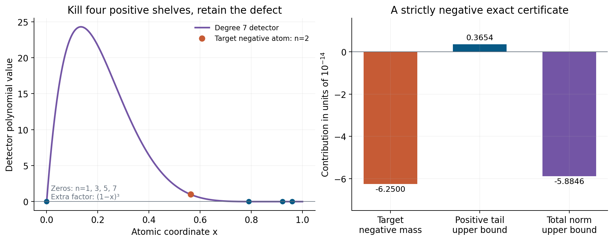
The detector vanishes on the first four positive shelves and equals one at the negative atom n=2. The positive bar is an upper bound for the entire remaining positive tail. The total upper bound is negative, so no omitted atom can reverse the conclusion.
The detector vanishes on the first four positive shelves and equals one at the negative atom \(n=2\). The positive bar is an upper bound for the entire remaining positive tail. The total upper bound is negative, so no omitted atom can reverse the conclusion.

View full-size figure (new tab)

The certificate uses rational arithmetic throughout

Take \(S=\{1,3,5,7\}\) and define

\[ P(x)=\prod_{n\in S}\frac{x-x_n}{x_2-x_n} \left(\frac{1-x}{1-x_2}\right)^3. \]

Its degree is seven. All remaining positive nodes begin at \(n=11\). With \(C=756482048/20777538825\) and \(r=3856/102487\), a complete tail bound gives

\[ Q_{10^{-12}}(P)\le-\frac{10^{-12}}{16} +\frac{C^2r^6}{3\cdot7^3} <-5.8845708899\times10^{-14}. \]

The inequality is certified as a comparison of exact rational numbers. The first four zeros remove the dominant positive contributions. The factor \((1-x)^3\) suppresses the remaining cluster near one. The construction exhibits a detecting degree, without asserting that degree seven is the smallest possible choice.

Passing every coarse test can still miss the defect

The previous witness would be less informative without a converse guarantee at lower resolution. For the same defect \(\delta=10^{-12}\), every nonzero polynomial of degree at most four has strictly positive quadratic form. This quantifies the information that the coarse test actually misses.
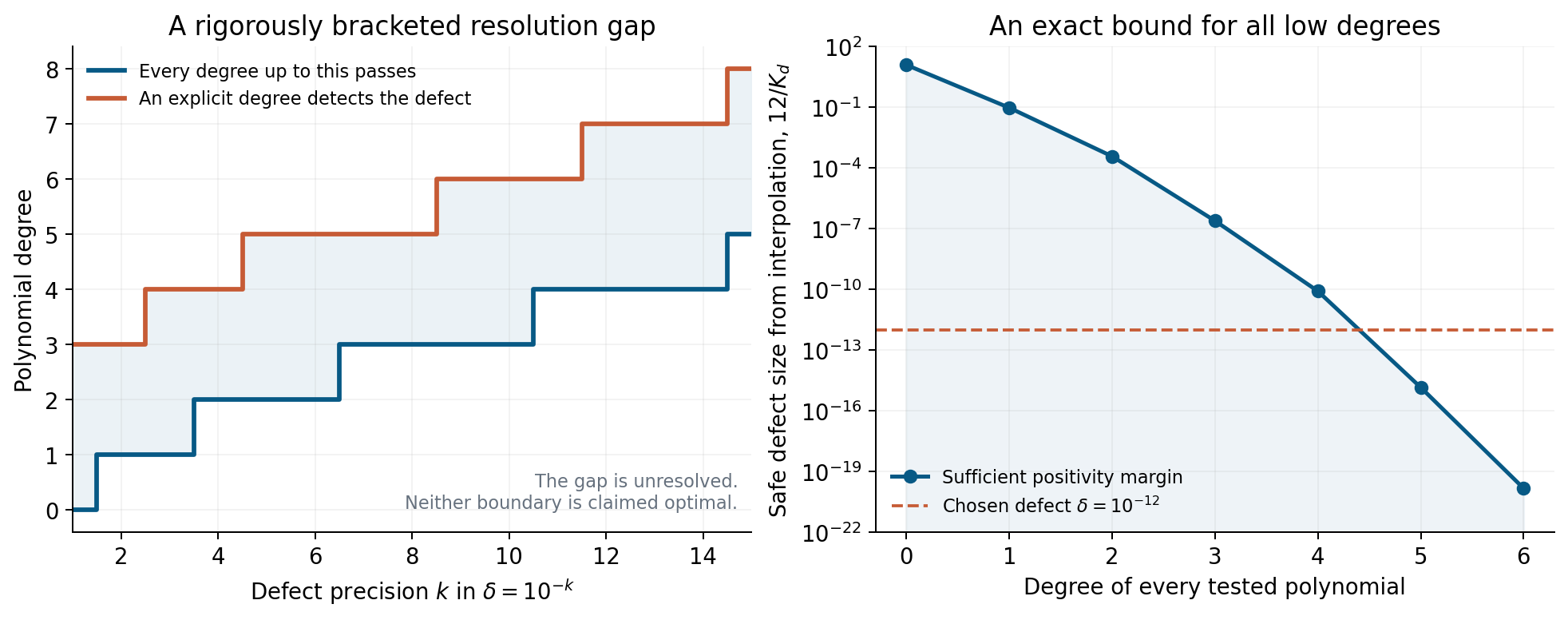
The blue boundary certifies positivity for every polynomial through that degree. The orange boundary gives an explicit detecting polynomial. The shaded gap remains unresolved by these certificates. At δ =10 -12 , degrees through four pass, degree seven fails, and degrees five and six are undecided here.
The blue boundary certifies positivity for every polynomial through that degree. The orange boundary gives an explicit detecting polynomial. The shaded gap remains unresolved by these certificates. At \(\delta=10^{-12}\), degrees through four pass, degree seven fails, and degrees five and six are undecided here.

View full-size figure (new tab)

Interpolation controls the whole polynomial space

Choose the odd squarefree labels \(n_i=1,3,5,7,11\), write \(y_i=x_{n_i}\), and put

\[ b_i=\prod_{j\ne i}\frac{\max(y_j,1-y_j)}{|y_i-y_j|}, \qquad K_4=\sum_{i=0}^{4}n_i^4b_i^2. \]

Lagrange interpolation and weighted Cauchy–Schwarz show that, for every polynomial \(f\) of degree at most four,

\[ Q_\delta(f)\ge \left(1-\frac{\delta K_4}{12}\right) \sum_{i=0}^{4}n_i^{-4}f(y_i)^2. \]

Exact rational comparison gives \(12/K_4>7.9790\times10^{-11}>10^{-12}\). A nonzero polynomial cannot vanish at all five selected nodes, so the right side is strictly positive. Thus the order-five Hankel matrix is positive definite, while the degree-seven witness makes the order-eight matrix fail positive semidefiniteness.

The complete atlas contains the general interpolation and detector bounds. Its reproducible check records 985 exact assertions and 16 floating algebra checks. The proofs establish the universal statements. The tests verify the stated finite certificates and implementations.

Source and conversion record

This HTML edition follows the retained manuscript. It adds no proof review or Lean coverage.

Source identities and equation checks

Notation in Special Functions

Look up a symbol without leaving this chapter. Select text before opening help to search for it.

Search this work’s notation.

    Symbols can have different meanings in different passages. Read each result in its own context.

    Open the full notation index