
Two functions exchange growth
For four real contractions \(0<q,r,a,b<1\), define the normalized pair
Each equation combines one value of \(U\) with one value of \(V\). The four scales specify where that exchange occurs. Both functions begin with the same unit slope, while later coefficients retain the two equations' different scale addresses.
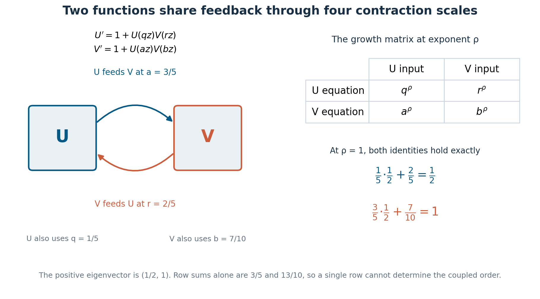
There is a unique entire solution pair. Both functions are odd, and every odd Taylor coefficient is positive. The common order is governed by the positive matrix
The eigenvector supplies the relative weights that a row sum misses. In the example, the row sums at \(s=1\) are \(3/5\) and \(13/10\). The coupled system nevertheless has order exactly one in both components.
The coefficients preserve both addresses
Write \(U(z)=\sum_{n\ge0}u_nz^{2n+1}\) and \(V(z)=\sum_{n\ge0}v_nz^{2n+1}\), with \(u_0=v_0=1\). The first equation gives the exact recursion
The second replaces \((q,r)\) by \((a,b)\) while retaining the same products \(u_i v_j\). Thus each new coefficient uses the shared history of the pair.
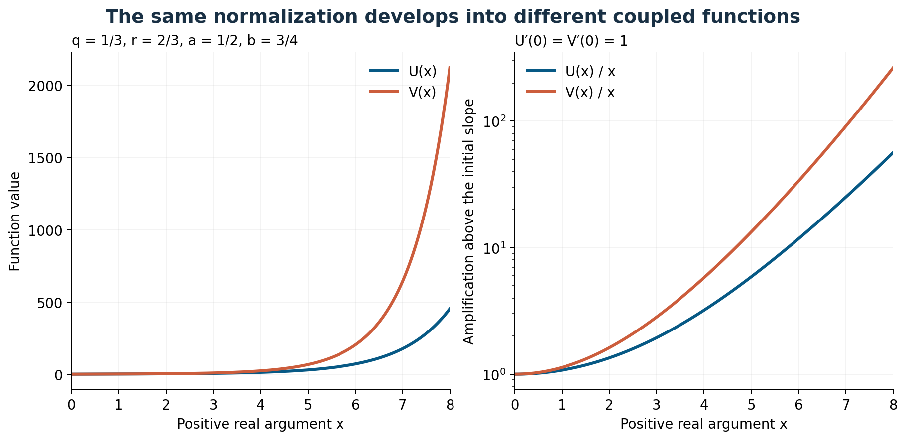
The first distinction already appears at degree three:
Induction gives \(0<u_n,v_n\le2^{-n}\), which supplies a convergent germ. If both functions are known on a disk of radius \(R\), their integral equations extend them to radius \(R/Q\), where \(Q=\max(q,r,a,b)<1\). Repeating this step reaches every finite disk.
The numerical agreement above checks the plotted approximation. The later certificate page supplies an exact bound on the omitted tail.
One order, two exact type proportions
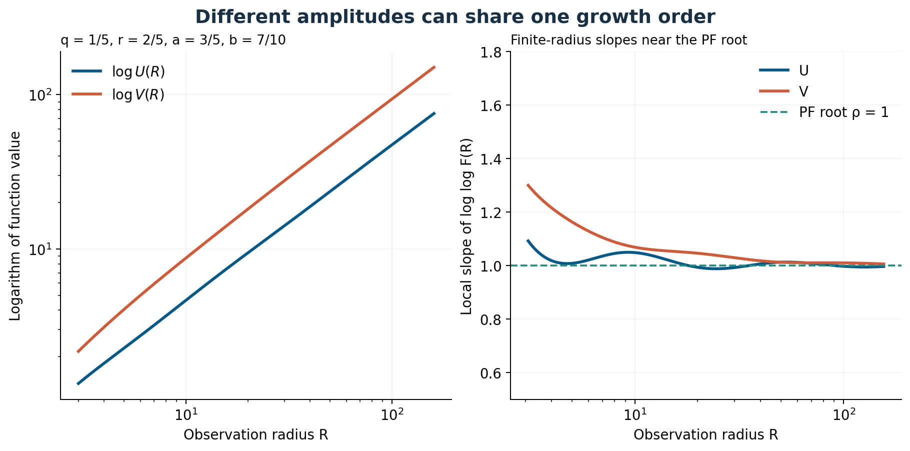
The entire functions have the same order \(\rho\), with positive lower type and finite upper type. Positivity places the maximum modulus on the positive real axis, so \(M_U(R)=U(R)\) and \(M_V(R)=V(R)\).
For \(F_1=U\) and \(F_2=V\), define
If \(P(\rho)w=w\) with \(w>0\), then both type vectors have precisely these Perron proportions:
For the worked pair, both the lower type and the upper type of \(V\) are twice the corresponding type of \(U\). Either both ordinary type limits exist or neither does. Equality of the lower and upper types remains open. The finite-radius slope picture does not decide that question.
Growth follows a spectral surface
The order is the unique positive solution of
The left side increases from zero to one as \(\rho\) increases. The right side decreases from one to zero. Their unique crossing determines the growth exponent without fitting a truncated Taylor curve.
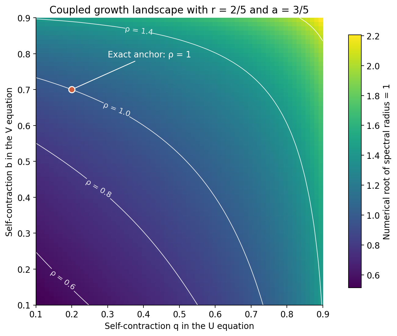
The order depends on the self scales \(q,b\) and on the product \(ar\) of the cross scales. Holding \(q,b,ar\) fixed preserves the order, while changing the cross scales separately generally changes the functions and their type proportions:
Consequently, equal order does not determine the family member. It fixes one growth exponent within a larger parameter space. The coefficients carry enough additional information to recover all four ordered scales away from the reduction surfaces described below.
A coefficient list with a certified tail
A finite Taylor list becomes an exact approximation certificate when it is paired with a bound on a larger disk. Let \(F\) be either component, and let \(F_N\) retain the odd indices \(0,\ldots,N\).
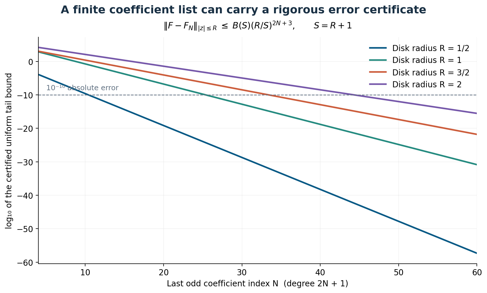
Put \(Q=\max(q,r,a,b)\). One elementary majorant starts with \(B(x)=x/(1-x^2)\) for \(0\le x<1\) and works outward through the finite contraction ladder using
The integral equations show that this bounds both components on the disk \(|z|\le x\). For \(S>R\ge0\), positivity then gives
The exponent is the first omitted odd degree. Every later term has an even smaller ratio between its values at radii \(R\) and \(S\). For the worked pair, \(N=30\), \(R=1\) and \(S=2\) give an error below \(1.600\times10^{-13}\) for both functions. The laboratory returns rational interval endpoints, so the certificate survives decimal rounding.
The phase calculus transports the pair
Use the derivative normalization \(A_n=(2n+1)!u_n\), \(B_n=(2n+1)!v_n\). Its recurrence has integer binomial weights:
The second component again replaces \((q,r)\) by \((a,b)\).
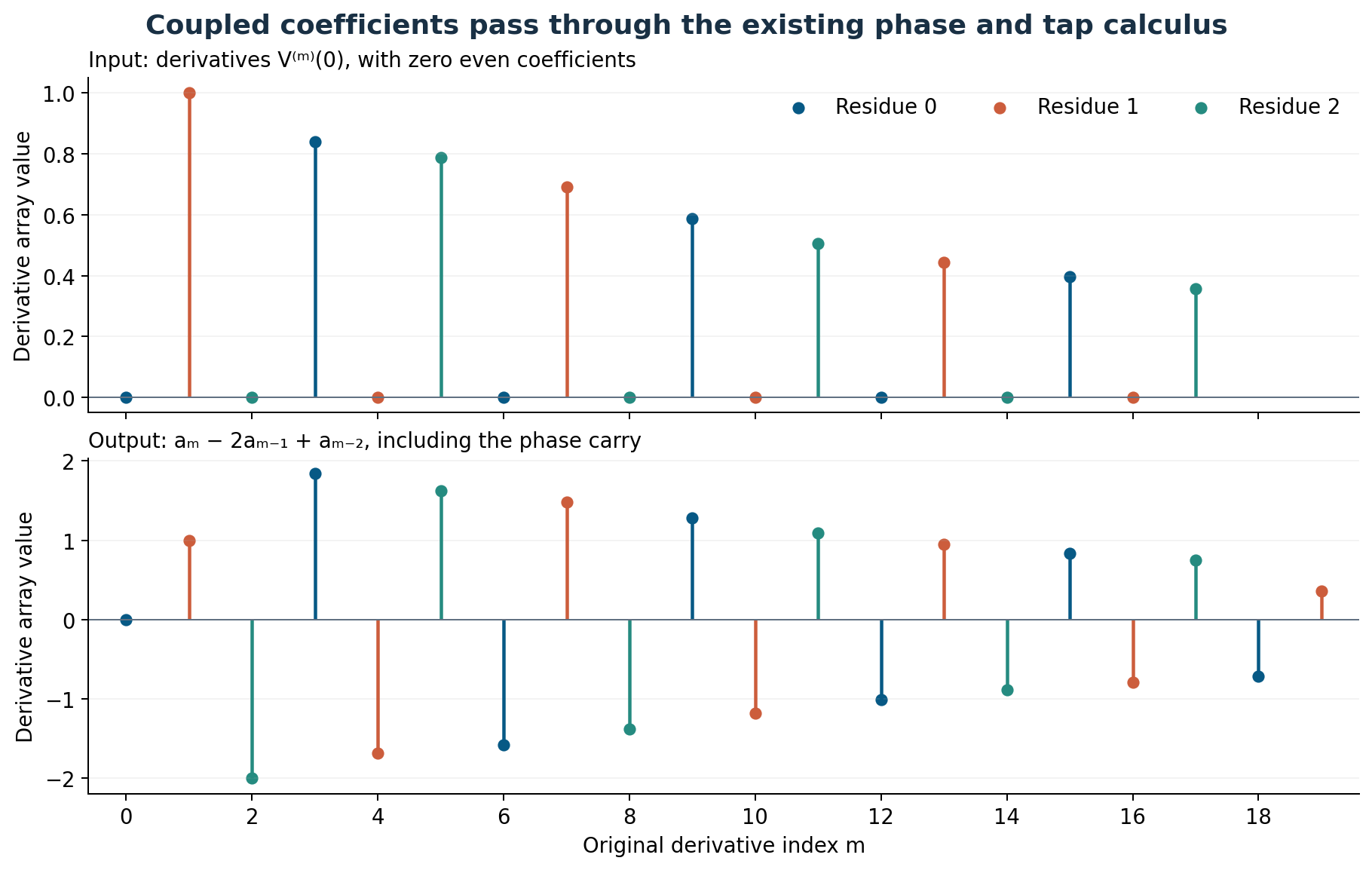
These derivative arrays are polynomials with nonnegative integer coefficients in the four scale variables. Their total degree is at most \(n(n+1)\). If every parameter denominator divides \(D_0\), then
This uniform clearing factor makes exact rational families available to integer sequence experiments. It need not be the smallest possible factor.
Ordinary taps on a derivative array correspond to repeated integration shifts of its exponential generating function. Multiplication of two exponential generating functions instead requires binomial convolution. The catalog preserves that distinction and marks generic integer and signed scale examples as formal series outside the proved analytic domain.
Two surfaces where one component rescales to the other
Set \(p=qr\), \(k=ab\), and use the ordinary Taylor coefficients \(u_2,v_2\) at degree five. The exact separation quantity factors as
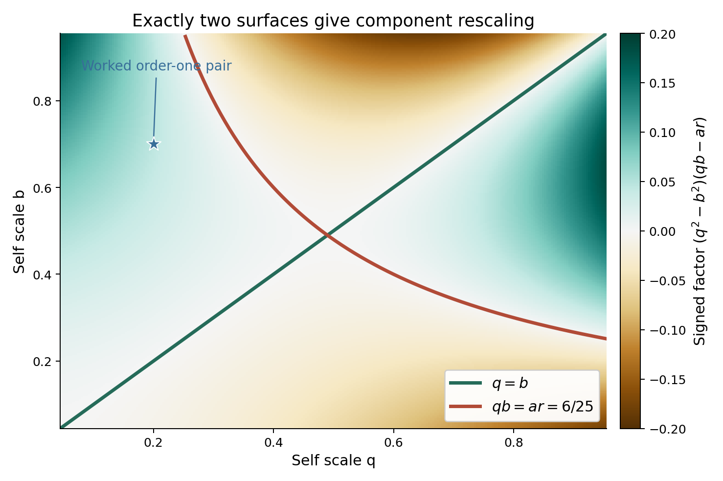
There exist nonzero complex constants \(A,B\) with \(V(z)=A\,U(Bz)\) if and only if \(D=0\). On either surface, put \(s=\sqrt{k/p}>0\). The scalar family is defined by \(T_{x,y}'(z)=1+T_{x,y}(xz)T_{x,y}(yz)\), \(T_{x,y}(0)=0\). It gives the explicit reduction
Both effective scales lie in \((0,1)\). Equality \(U=V\) is more restrictive: it occurs exactly when \(\{q,r\}=\{a,b\}\).
This classifies relations between the normalized components. Separately, no invertible constant linear coordinate change decouples the defining operator into two autonomous scalar equations on every analytic input. That operator statement does not exclude nonlinear changes of variables or other special-function identities.
Degree seven identifies the four scales
Away from \(D=0\), the six coefficients \((u_1,v_1,u_2,v_2,u_3,v_3)\) uniquely recover the ordered parameters \((q,r,a,b)\) in \((0,1)^4\). These are the coefficients at degrees three, five and seven of the two labeled functions.
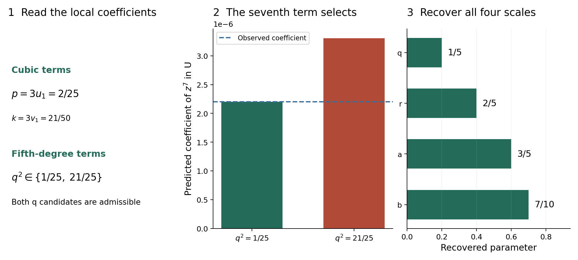
First \(p=3u_1\) and \(k=3v_1\). The possible values \(x=q^2\) and \(y=a^2\) satisfy
For two distinct positive candidates \(x,x'\), the predicted seventh coefficients differ by
The second component supplies the analogous separation for \(y\). Finally take the positive square roots and recover \(r=p/q\), \(b=k/a\).
This is an exact-data inverse theorem. Near a reduction surface, small \(D\) can make candidate predictions close, so a uniform stable inverse does not follow. The degree-seven recovery and the reduction classification are proved statements. Historical priority of these particular results is addressed separately by the bounded literature comparison.