
Write the split dynamics as \(y_{t+1}=Ay_t+Bw_t\) and \(w_{t+1}=Cy_t+Dw_t\). Eliminating \(w_t\) gives
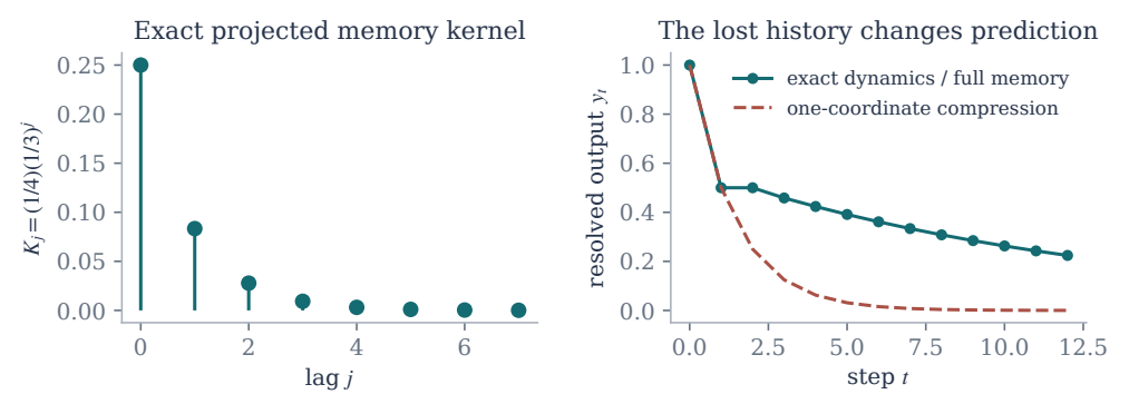
Read the diagram in words
The kernel plot describes the contribution of older resolved states after the discarded coordinate has been eliminated. The trajectory comparison uses the declared rational example. A tail bound evaluated on the true history and an error bound for a recursively generated prediction are different statements; the text keeps their assumptions separate.
For the running example, \(A=1/2\), \(B=1\), \(C=1/4\), \(D=1/3\) and \(w_0=0\). Thus \(K_j=\tfrac14\,3^{-j}\). If \(|y_t|\leq1\), retaining the last \(H\) history terms leaves a same-history tail at most \(\Delta_H=\tfrac38\,3^{-H}\).
Here \(0\leq y_t\leq1\) and the truncated recursion has gain
With the same initial state, recursive propagation therefore gives
Scope
P10's tail estimate uses the same resolved history. P19 supplies the separate stability argument for a predictor using its own history. For other initial states, retain the term \(BD^tw_0\).