
I.6 Moving packets, connections, and curvature
On this page · Permalink · Source line 464
I.6.1 Moving quantum coordinates
On this page · Permalink · Source line 466
Theorem I.6.1: Moving-frame Hamiltonian
Let \(U(t)\) and \(\psi(t)\) be differentiable on an open real time interval, let \(U(t)\) be unitary, and let \(H(t)=H(t)^*\). Suppose
Writing
gives
Both the connection term \(-iU^*\dot U\) and the effective Hamiltonian \(U^*HU-iU^*\dot U\) are Hermitian.
Read proof · Read statement and proof side by side · Permalink · Source line 468 · Claim record · Lean coverage · Code · Worked examples
Proof of Theorem I.6.1
Differentiate \(\psi=Uy\):
Multiplying by \(U^*\) gives the formula. Differentiating \(U^*U=I\) shows \(U^*\dot U\) is skew-Hermitian, so \(-iU^*\dot U\) is Hermitian.
Back to statement · Read statement and proof side by side · Permalink · Source line 488 · Claim record · Lean coverage · Code · Worked examples
Text description
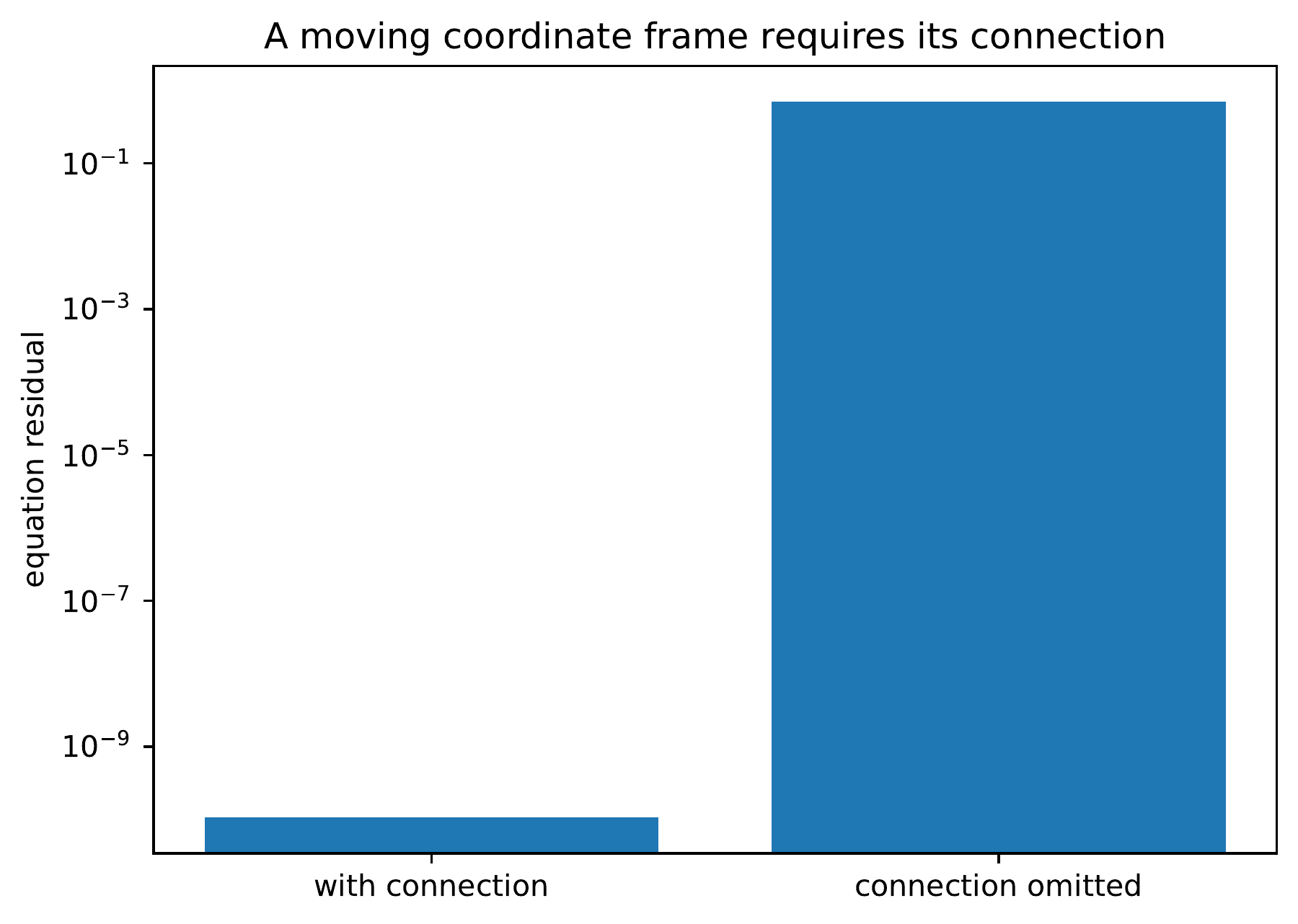
Two bars use a logarithmic residual axis. Retaining the connection gives a residual near numerical precision; omitting it gives a much larger residual. The comparison isolates the connection term in the moving-coordinate equation.
Numerical certificate I.6.2: Moving-frame correction
The reported residual for the complete equation in the moving frame was \(1.0645\times10^{-10}\). Omitting the connection increased the residual to \(0.7000\).
Permalink · Source line 503 · Claim record · Lean coverage · Code · Worked examples
I.6.2 A canonical projector connection
On this page · Permalink · Source line 507
Let \(P_1(t),\ldots,P_m(t)\) be differentiable on an open real time interval, with \(P_a(t)^*=P_a(t)\) and
Theorem I.6.3: Canonical packet connection
Define
Then
and
for every packet \(b\).
Read proof · Read statement and proof side by side · Permalink · Source line 516 · Claim record · Lean coverage · Code · Worked examples
Proof of Theorem I.6.3
Differentiating \(P_a^2=P_a\) gives
Summing over \(a\) and using \(\sum_a\dot P_a=0\) yields
which proves both displayed formulas for \(C\) and its skew-Hermiticity.
For fixed \(b\),
When \(a\ne b\), differentiating \(P_bP_a=0\) gives
Hence
and subtraction gives \([C,P_b]=\dot P_b\).
Back to statement · Read statement and proof side by side · Permalink · Source line 540 · Claim record · Lean coverage · Code · Worked examples
The connection generates infinitesimal transport of the moving packet frame. The packet family determines it directly, so its construction does not require a basis inside any packet.
I.6.3 Projector curvature
On this page · Permalink · Source line 570
Classical input I.6.4: Projected connection
Let \(M\) be a smooth finite-dimensional real manifold without boundary, let \(V\) be a finite-dimensional real normed vector space, and let \(P:M\to\operatorname{End}_{{\mathbb R}}(V)\) be smooth with \(P(x)^2=P(x)\). In the quantum application, \(V\) is the underlying real space of a finite complex Hilbert space and \(P\) is an orthogonal complex-linear projector.
The rank of \(P\) is locally constant. On each open rank region, its ranges form a smooth vector bundle. For a smooth range section \(s\), so that \(Ps=s\), define
This is a connection on smooth range sections. For smooth vector fields \(X,Y\), its curvature satisfies
Equivalently, its endomorphism-valued curvature is
No global frame or globally constant rank is required, and the vector fields need not commute. The geometric formalization concerns real smooth structures. It does not cover complex analytic manifolds or extensions to a boundary.
Read proof · Read statement and proof side by side · Permalink · Source line 572 · Claim record · Lean coverage · Code · Worked examples
Proof of Classical input I.6.4
Range coordinates. Fix \(a\in M\) and put
Then \(T_a(a)=I\) and \(P(x)T_a(x)=T_a(x)P(a)\). Invertibility is open, so on a neighborhood of \(a\), \(T_a(x)\) restricts to an isomorphism from \({\operatorname{Ran}} P(a)\) to \({\operatorname{Ran}} P(x)\). This proves local constancy of rank. The local coordinates and their transitions are
Their smoothness follows from smoothness of \(P\) and inversion. The transition maps satisfy the cocycle identity by cancellation. These charts construct the smooth range bundles on the open rank regions, including when different connected components have different ranks.
Connection rules. Smoothness of \(P\,ds(X)\) and \(P^2=P\) show that \(\nabla_Xs\) is a smooth range section. Differentiation and projection give
for smooth real \(f\). The range coordinates above identify ambient smooth range sections with smooth sections of the constructed bundle.
Curvature. Differentiating \(P^2=P\) gives \(P(dP(X))P=0\). Write \(D_Xs=ds(X)\). For ambient smooth sections,
Expansion of the projected derivatives therefore leaves
Since \(Ps=s\), differentiation gives \(D_Ys=(dP(Y))s+PD_Ys\). The terms with a middle \(P\) vanish. Thus
This expression is alternating and bilinear in the tangent vectors, and it preserves the range. The ordinary chain rule and the transformation law for the Lie bracket make the local calculations agree on chart overlaps, which gives the global formula.
Back to statement · Read statement and proof side by side · Permalink · Source line 593 · Claim record · Lean coverage · Code · Worked examples
For an orthogonal rank-one complex projector, use the scalar connection convention \(A=-i\langle u,du\rangle\) in a local unit frame. The associated scalar curvature density is
On the Bloch sphere,
where
The Pauli multiplication law gives
Using \({\operatorname{Tr}}(P\,\mathbf a\cdot\boldsymbol\sigma)=\mathbf n\cdot\mathbf a\) therefore yields
The scalar sign changes if the opposite convention for \(A\) is chosen. This explicit calculation is not a separate entry among the 19 items in the Lean register.
Text description
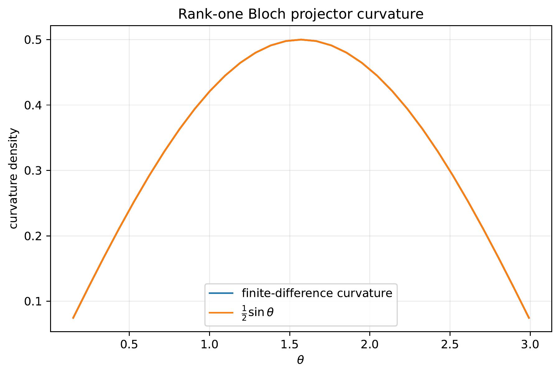
The plot compares the finite-difference curvature and the exact one-half sine-of-theta curve over the displayed polar-angle interval. Both rise to a central peak and fall to zero at the endpoints, with the curves visually coincident at this scale.
Numerical certificate I.6.5: Geometric packet identities
The canonical connection reconstructed every packet derivative with residual \(0\). The maximum residual for the Bloch curvature was \(2.0803\times10^{-11}\).
Permalink · Source line 666 · Claim record · Lean coverage · Code · Worked examples