
I.4 Quantum circuits as packet paths
On this page · Permalink · Source line 273
Let
be a circuit with \(m\ge1\), and let \(\{P_\alpha\}\) be a complete packet system. For the empty circuit \(m=0\), set \(U=I\). Its boundary block is \(P_\beta P_\alpha=\delta_{\beta\alpha}P_\alpha\).
Theorem I.4.1: Exact circuit path expansion
For source packet \(\alpha_0\) and target packet \(\alpha_m\),
Summing over the source and target packets reconstructs the complete circuit operator.
Read proof · Read statement and proof side by side · Permalink · Source line 281 · Claim record · Lean coverage · Code · Worked examples
Proof of Theorem I.4.1
Insert the identity resolution \(I=\sum_\alpha P_\alpha\) between every adjacent pair of gates. Distributing the finite sums gives the path expansion. Summing the left and right boundary projectors reconstructs \(U\).
Back to statement · Read statement and proof side by side · Permalink · Source line 296 · Claim record · Lean coverage · Code · Worked examples
Theorem I.4.2: Packetwise unitarity conservation
If \(U\) is unitary and \(U_{\beta\alpha}=P_\beta UP_\alpha\), then
Similarly,
Read proof · Read statement and proof side by side · Permalink · Source line 300 · Claim record · Lean coverage · Code · Worked examples
Proof of Theorem I.4.2
Using completeness and unitarity,
For the second identity, sum over the source packets and use unitarity in the reverse order.
Back to statement · Read statement and proof side by side · Permalink · Source line 317 · Claim record · Lean coverage · Code · Worked examples
Example I.4.3: Bell seed circuit
In this example only, \(H\) denotes the Hadamard gate, not a Hamiltonian. Starting from \({\left|00\right\rangle}\),
and then
The parity packets show that the final state lies entirely in the even sector, while the intermediate circuit path passes through both even and odd addresses.
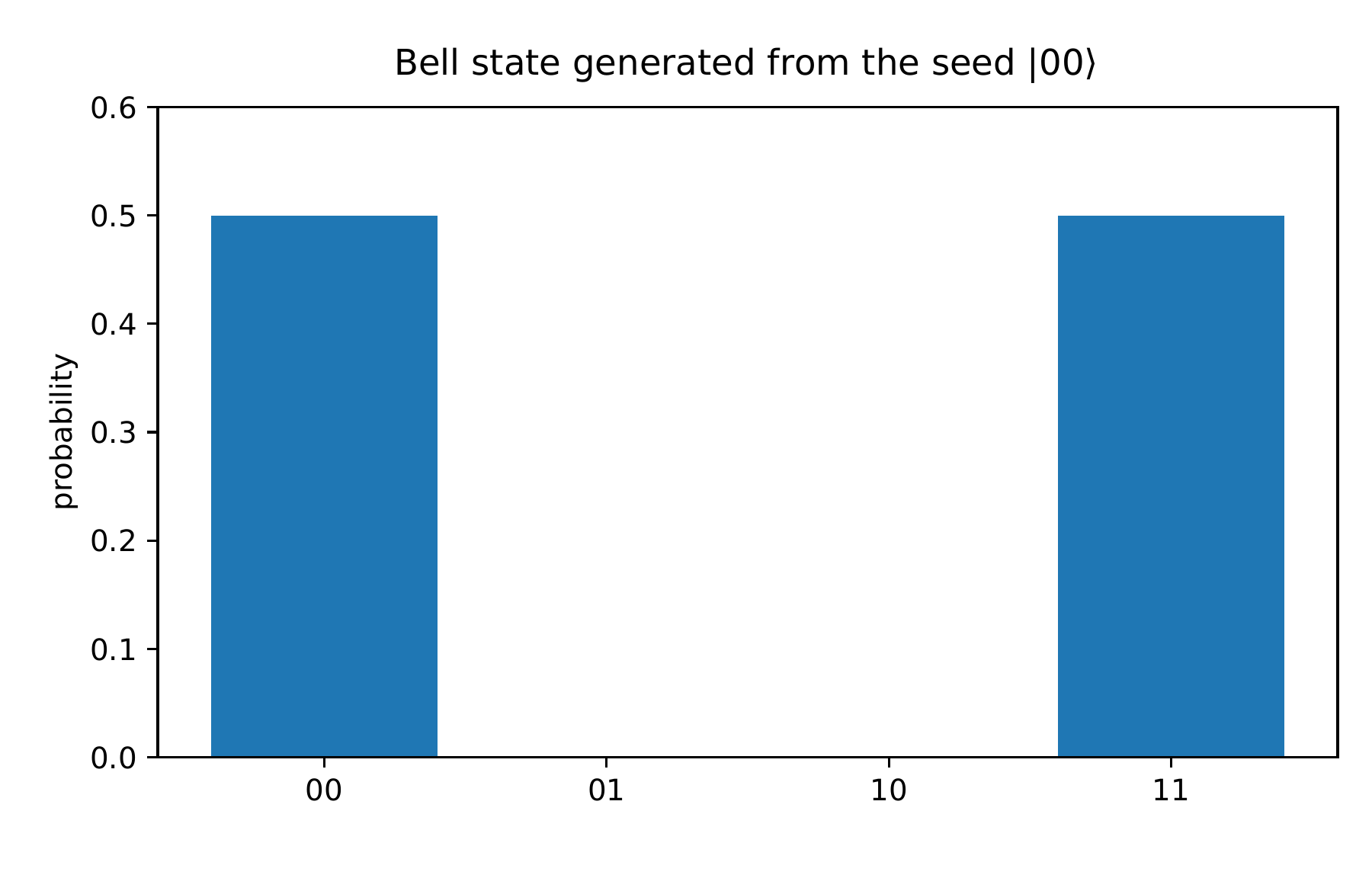
Text description
The bar chart has four computational addresses: 00, 01, 10, and 11. The bars at 00 and 11 have height one half; the other two have height zero. This is the displayed Bell state prepared from the 00 seed.
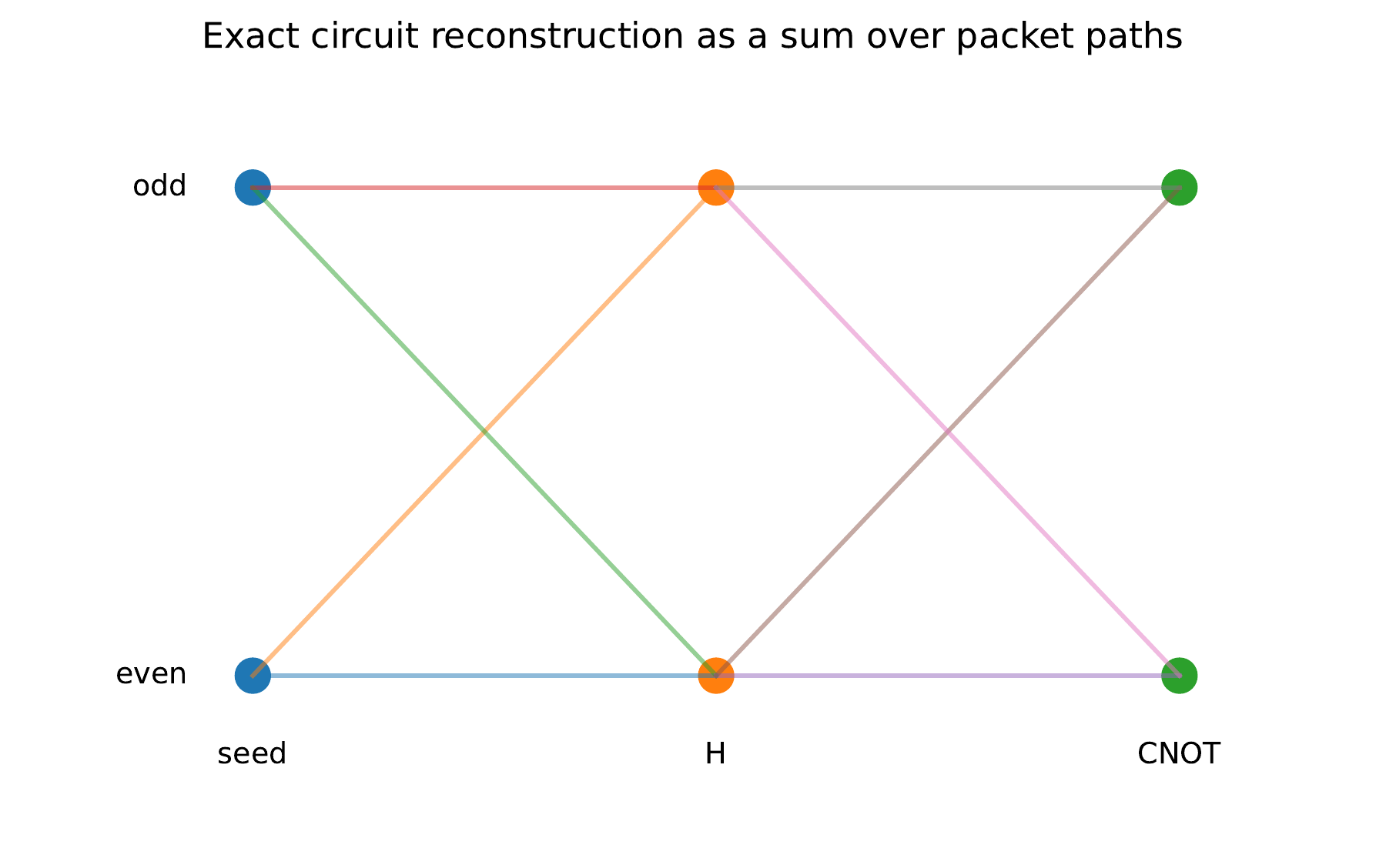
Text description
The horizontal axis shows seed, H, and CNOT stages. Each stage has even and odd packet nodes, with colored links indicating possible transfers between them. Summing the path contributions reconstructs the circuit action.
Numerical certificate I.4.4: Bell and path reconstruction
The original numerical implementation reported residuals of \(0\) for both the Bell state and its complete reconstruction from parity paths.
Permalink · Source line 361 · Claim record · Lean coverage · Code · Worked examples