1 Coefficient conventions, logical status, and scope
On this page · Permalink · Source line 1
Reader roadmap
This section sets out the conventions used throughout the paper. It explains when a statement concerns algebra, when topology enters the argument, which results are taken as classical input, and how the stable record IDs connect this paper to later work. Keeping these settings distinct makes the hypotheses of each result easier to follow.
1.1 Ambient regimes and theorem records
On this page · Permalink · Source line 5
Definition 1.1: Coefficient and module regimes
All modules are left modules unless stated otherwise. The algebraic regime consists of a unital ring \(A\) and a unital left module \(M\) over \(A\). When linear dimensions, tensor products, quivers, or operator blocks are used, \(A\) is a unital algebra over \({\Bbbk}\), where \({\Bbbk}\) is a field, and \(M\) is a vector space over \({\Bbbk}\). The topological regime consists of a Hausdorff topological vector space over a complete valued field, together with a unital algebra of continuous linear operators. Every infinite sum, completion, quotient topology, and closure below is interpreted only in the regime explicitly declared in its statement.
Permalink · Source line 7 · Claim record · Lean coverage · Code · Worked examples
Conventions for empty families.
On this page · Permalink · Source line 12
For finite families of nonnegative integers we use \(\max\varnothing=0\). The height of an empty finite partially ordered set is \(0\), as is the height of a nonempty poset with no strict comparable pair. Thus the height in the theorem for the support preorder counts strict steps.
Definition 1.2: Canonical theorem record
A canonical theorem record is the tuple
A downstream paper cites the stable record ID. A domain specialization may add domain hypotheses, but it does not repeat a generic proof from this paper.
Permalink · Source line 14 · Claim record · Lean coverage · Code · Worked examples
Boundary 1.3: Symbolic scope
This edition proves the algebraic and topological statements printed below. It does not assert historical novelty, independent external certification, automatic discovery of useful packet systems, nonlinear obstruction theory, multilevel refinement, arithmetic congruences, quantum gravity, automorphy, or local or global Langlands reciprocity.
Permalink · Source line 25 · Claim record · Lean coverage · Code · Worked examples
2 Typed operator grammars, realizations, and seed systems
On this page · Permalink · Source line 31
Reader roadmap
An operator grammar describes which compositions are allowed and which relations they satisfy. A realization gives this syntax a concrete action on vector spaces. Its realized algebra consists of the operators that actually occur in that action. We can then ask which vectors serve as seeds.
2.1 Typed syntax and module realizations
On this page · Permalink · Source line 35
Definition 2.1: Typed operator grammar
Let \(Q=(Q_0,Q_1,s,t)\) be a quiver with finite vertex set. A typed operator grammar over \({\Bbbk}\) is a pair
where \(I\triangleleft {\Bbbk} Q\) is an ideal on both sides generated by linear combinations over \({\Bbbk}\) of paths having common source and common target. Write
A realization of \(\mathfrak G\) is a family \((X_v)_{v\in Q_0}\) and linear maps
that annihilate every relation in \(I\). A morphism \(f:X\to Y\) of realizations is a family of linear maps \(f_v:X_v\to Y_v\) satisfying
Visual guide: An atlas of the objects · Permalink · Source line 37 · Claim record · Lean coverage · Code · Worked examples
Definition 2.2: Realization on a single space
For a typed realization \(X\), define its realization on a single space by
Every vertex idempotent acts as a coordinate projector on \(|X|\), and every path acts as a block operator from its source space to its target space.
Permalink · Source line 60 · Claim record · Lean coverage · Code · Worked examples
Theorem 2.3: Typed realization and module equivalence
The category of realizations of \(\mathfrak G\) is equivalent to the category of unital left modules over \(\Lambda_{\mathfrak G}\). Explicitly, a realization \(X\) determines the collapsed space \(|X|\) of Definition 2.2 with the vertex idempotent \(e_v\) acting as the coordinate projector onto \(X_v\) and each arrow acting in the block between its declared source and target. Conversely, a unital module \(M\) over \(\Lambda_{\mathfrak G}\) determines the realization
The two constructions are inverse up to canonical natural isomorphism.
Read proof · Read statement and proof side by side · Permalink · Source line 70 · Claim record · Lean coverage · Code · Worked examples
Proof of Theorem 2.3
Because \(Q_0\) is finite, \(1=\sum_{v\in Q_0}e_v\) in \({\Bbbk} Q\), the \(e_v\) are pairwise orthogonal, and the same identities hold in \(\Lambda_{\mathfrak G}\). Given a realization, define the action of a path by composition of its arrow maps and extend linearly. Every element of \(I\) acts as zero, so the action factors through \(\Lambda_{\mathfrak G}\). The vertex idempotents give
Conversely, if \(M\) is unital, then
Orthogonality makes the sum direct. For an arrow \(a:v\to w\), the identities \(a=e_wae_v\) imply
The relations in \(I\) act as zero because \(M\) is a module over \(\Lambda_{\mathfrak G}\). Applying both constructions returns the original vertex spaces and arrow maps, or the original module decomposition, through the evident identity maps. These identifications commute with morphisms, giving an equivalence of categories.
Back to statement · Read statement and proof side by side · Permalink · Source line 84 · Claim record · Lean coverage · Code · Worked examples
How to read the result
The equivalence does not claim that a quiver presentation is unique. It says that once a grammar is fixed, working with typed arrows and working with a module over the quotient path algebra carry the same information. The typed description is often easier for constructing an operator system. The module description is often easier for proving generation and quotient theorems.
A grammar with two vertices
Take two vertices and one arrow \(a:1\to2\). A realization is simply a pair of spaces and a linear map
After collapse, \(|X|=X_1\oplus X_2\), the vertex idempotents are the two coordinate projectors, and \(a\) is a single block outside the diagonal. This elementary case already contains the viewpoint of packets and transfer blocks used later.
2.2 The realized action and faithful reduction
On this page · Permalink · Source line 113
Definition 2.4: Realized operator algebra
For a realization \(X\), the realized operator algebra is
It records the actual operators in the realization and may be a proper quotient of the abstract grammar algebra.
Permalink · Source line 114 · Claim record · Lean coverage · Code · Worked examples
Proposition 2.5: Action factorization and hull invariance
Let \(S\subseteq |X|\). The generated submodule under the grammar algebra equals the generated submodule under the realized operator algebra:
Consequently, every statement about seed rank depends only on the realized action, not on redundant relations in a chosen presentation of the grammar.
Read proof · Read statement and proof side by side · Permalink · Source line 124 · Claim record · Lean coverage · Code · Worked examples
Proof of Proposition 2.5
The action map \(\rho:\Lambda_{\mathfrak G}\twoheadrightarrow{\mathcal A}_X\) is surjective by definition and satisfies \(\lambda s=\rho(\lambda)s\). Hence every grammar orbit vector lies in \({\mathcal A}_XS\). The reverse inclusion holds because every element of \({\mathcal A}_X\) is \(\rho(\lambda)\) for some \(\lambda\).
Back to statement · Read statement and proof side by side · Permalink · Source line 135 · Claim record · Lean coverage · Code · Worked examples
The central idea
Replacing the abstract grammar algebra by its image \({\mathcal A}_X\) removes syntax that acts as zero. This is a faithful reduction of the action. It does not change any orbit, hull, or computation of seed rank.
2.3 Seeds, addressed hulls, and natural presentations
On this page · Permalink · Source line 144
Definition 2.6: Linear seed system
A linear seed system is a tuple
where \(X\) is a unital left module over \({\mathcal A}\), \({\mathcal A}\) is fixed independently of the target element, \(S=(s_1,\ldots,s_r)\) is a finite distinguished seed family, \({\mathcal P}\) is either empty or a declared packet system, and \(\tau\) is either the algebraic convention or a specified Hausdorff topology in which the declared operator action is continuous.
Visual guide: An atlas of the objects · Permalink · Source line 145 · Claim record · Lean coverage · Code · Worked examples
Definition 2.7: Generated hull
For \(S\subseteq X\), define
In the topological regime define
For a singleton \(S=\{s\}\), write \({\operatorname{Hull}}_{{\mathcal A}}(s)\).
Permalink · Source line 155 · Claim record · Lean coverage · Code · Worked examples
The algebraic hull uses finite sums of addressed seed vectors. In the topological setting, taking its closure may add limits that no finite expression reaches. Thus algebraic generation and dense generation answer different questions, even when they use the same seeds and operators.
Definition 2.8: Natural presentation
A seed presentation is natural relative to a declared grammar when the primitive operators and relations are fixed independently of the target, the relation system is finite or effectively enumerable, the topology is intrinsic to the realization, no primitive operator directly stores the complete target, and the presentation exposes a reusable invariant, theorem, or computation not encoded by a primitive chosen for the target.
Permalink · Source line 171 · Claim record · Lean coverage · Code · Worked examples
Proposition 2.9: Algebra generation and module generation are distinct
Every nonzero unital algebra \(A\), regarded as a left module over itself, has
with cyclic seed \(1_A\). This conclusion is independent of the number of algebra generators required to present \(A\) as an algebra.
Read proof · Read statement and proof side by side · Permalink · Source line 177 · Claim record · Lean coverage · Code · Worked examples
Proof of Proposition 2.9
For every \(a\in A\), one has \(a=a1_A\). Hence \(A1_A=A\). The number of operations needed to generate \(A\) as an algebra is a different invariant and does not enter the module calculation.
Back to statement · Read statement and proof side by side · Permalink · Source line 188 · Claim record · Lean coverage · Code · Worked examples
Boundary 2.10: Operators chosen for a target
For a fixed seed \(s\) and target \(x\), the existence of a specially defined operator \(A_x\) satisfying \(A_xs=x\) does not establish a natural seed calculus unless \(A_x\) belongs to a grammar fixed independently of the target satisfying Definition 2.8.
Permalink · Source line 192 · Claim record · Lean coverage · Code · Worked examples
Do not conflate
An operator may be chosen because it sends the current seed to a desired target. Such a choice proves only an existence statement for that one target unless the operator already belongs to the fixed algebra. The algebra must be declared before the question of seed rank is asked. Otherwise the acting system changes with the answer one wants to obtain.

3 Free presentations by seeds and relations
On this page · Permalink · Source line 210
Reader roadmap
A seed family gives a canonical map from a finite free module. The generated hull is exactly its image, and the relations among addressed seeds form the kernel. This converts orbit generation into a presentation problem.
3.1 Finite free covers
On this page · Permalink · Source line 214
Definition 3.1: Seed evaluation map
Let \(A\) be a unital ring, let \(M\) be a left module over \(A\), and let \(S=(s_1,\ldots,s_r)\in M^r\). Define the linear map over \(A\)
Permalink · Source line 215 · Claim record · Lean coverage · Code · Worked examples
Theorem 3.2: Finite free presentation
For the map in Definition 3.1,
and the induced map is an isomorphism of left modules over \(A\)
Consequently, \(S\) generates \(M\) if and only if \(\varepsilon_S\) is surjective.
Read proof · Visual guide: Relations identify words, not just outputs · Read statement and proof side by side · Permalink · Source line 226 · Claim record · Lean coverage · Code · Worked examples
Proof of Theorem 3.2
The image consists exactly of finite sums \(\sum_ja_js_j\), which is \({\operatorname{Hull}}_A(S)\). Because \(\varepsilon_S\) is linear over \(A\), its kernel is a left submodule. The first isomorphism theorem gives
The final equivalence is the equality \({\operatorname{im}}\varepsilon_S=M\).
Back to statement · Read statement and proof side by side · Permalink · Source line 244 · Claim record · Lean coverage · Code · Worked examples
How to read the result
The theorem converts the geometric language of addressed seed orbits into the algebraic language of generators and relations. A word in the operators is represented by an element of the free module. Two addressed expressions represent the same vector exactly when their difference lies in the kernel. The generated hull is therefore not merely spanned by the free module. It is its canonical quotient.
A cyclic nilpotent chain
Let \(A={\Bbbk}[t]\) and \(M={\Bbbk}[t]/(t^3)\). The residue class \(s=[1]\) is one seed and
has kernel \((t^3)\). Hence \(M\cong A/(t^3)\), and the addressed vectors \(s,ts,t^2s\) are the visible orbit chain.
Corollary 3.3: Characterization by minimal free covers
For every finitely generated left module \(M\) over \(A\),
Read proof · Read statement and proof side by side · Permalink · Source line 267 · Claim record · Lean coverage · Code · Worked examples
Proof of Corollary 3.3
A seed family of size \(r\) gives a surjection by Theorem 3.2. Conversely, the images of the standard basis vectors under any surjection \(A^{\oplus r}\twoheadrightarrow M\) form a generating family of size at most \(r\).
Back to statement · Read statement and proof side by side · Permalink · Source line 279 · Claim record · Lean coverage · Code · Worked examples
Corollary 3.4: Presentation with one seed
For \(s\in M\), the annihilator
is a left ideal and
Read proof · Visual guide: Relations identify words, not just outputs · Read statement and proof side by side · Permalink · Source line 283 · Claim record · Lean coverage · Code · Worked examples
Proof of Corollary 3.4
The evaluation map for one seed is \(a\mapsto as\). Its kernel is \(\operatorname{Ann}_A(s)\), which is therefore a left ideal, and Theorem 3.2 gives the quotient isomorphism.
Back to statement · Read statement and proof side by side · Permalink · Source line 297 · Claim record · Lean coverage · Code · Worked examples
3.2 One seed and the distinction between module and algebra relations
On this page · Permalink · Source line 301
Proposition 3.5: Criterion for the annihilator to be an ideal on both sides
For \(s\in M\), the left ideal \(L=\operatorname{Ann}_A(s)\) is an ideal on both sides if and only if
If \(s\) is cyclic, these conditions are equivalent to
Read proof · Visual guide: Relations identify words, not just outputs · Read statement and proof side by side · Permalink · Source line 302 · Claim record · Lean coverage · Code · Worked examples
Proof of Proposition 3.5
The left ideal \(L\) is an ideal on both sides exactly when \(ab\in L\) for every \(a\in L\) and \(b\in A\). This is equivalent to
By additivity, the last identity is equivalent to \(L{\operatorname{Hull}}_A(s)=0\).
If \(s\) is cyclic, then \({\operatorname{Hull}}_A(s)=M\). Hence the preceding condition is \(L\subseteq\operatorname{Ann}_A(M)\). The reverse inclusion always holds because an operator annihilating all of \(M\) annihilates \(s\). Thus equality follows. Conversely, \(\operatorname{Ann}_A(M)\) is an ideal on both sides, so equality implies that \(L\) is an ideal on both sides.
Back to statement · Read statement and proof side by side · Permalink · Source line 316 · Claim record · Lean coverage · Code · Worked examples
Why a seed annihilator need not be an ideal on both sides
Let \(A=M_2({\Bbbk})\) act on \(M={\Bbbk}^2\), and let \(s=e_1\). Then \(\operatorname{Ann}_A(s)\) consists of matrices whose first column is zero. It is a left ideal because left multiplication preserves a zero first column. It is not generally a right ideal. Thus the natural quotient for one seed is a quotient of the left regular module, not automatically a quotient algebra.
3.3 Topological completion of a presentation
On this page · Permalink · Source line 332
Theorem 3.6: Completion of a dense free presentation
Let \(X\) be a complete Hausdorff locally convex space, let \({\mathcal A}\subseteq{\operatorname{End}}(X)\) act continuously, and let \(S=(s_1,\ldots,s_r)\). Put
algebraically and let \(j:E\to X\) be the injective map induced by \(\varepsilon_S\). Give \(E\) the locally convex topology transported from \(j(E)\), equivalently the topology generated by
for the continuous seminorms \(p\) on \(X\). Every \(a\in{\mathcal A}\) acts continuously on \(E\) in the transported topology and therefore extends to \(\widehat E\). If \({\operatorname{Hull}}_{{\mathcal A}}(S)\) is dense in \(X\), then \(j\) extends uniquely to a topological isomorphism of modules over \({\mathcal A}\)
Read proof · Visual guide: Density is not finite generation of each vector · Read statement and proof side by side · Permalink · Source line 333 · Claim record · Lean coverage · Code · Worked examples
Proof of Theorem 3.6
By Theorem 3.2, \(j\) is an algebraic isomorphism of modules over \({\mathcal A}\) from \(E\) onto \({\operatorname{Hull}}_{{\mathcal A}}(S)\). The transported seminorms make it a topological isomorphism onto that subspace. For \(a\in{\mathcal A}\) and a continuous seminorm \(p\) on \(X\), continuity of \(a:X\to X\) supplies continuous seminorms controlling \(p(aj(e))\), so the induced action on \(E\) is continuous and extends uniquely to \(\widehat E\). The subspace is dense by hypothesis. A Cauchy net in \(E\) is mapped to a Cauchy net in \(X\), which converges because \(X\) is complete. This defines a continuous extension \(\widehat j:\widehat E\to X\). For any \(x\in X\), choose a net \((e_\lambda)\) in \(E\) with \(j(e_\lambda)\to x\). The transported topology makes \((e_\lambda)\) Cauchy, so it converges to some \(\xi\in\widehat E\), and continuity gives \(\widehat j(\xi)=x\). Thus \(\widehat j\) is surjective. If \(\widehat j(\xi)=0\), represent \(\xi\) by a Cauchy net \((e_\lambda)\). Then \(j(e_\lambda)\to0\), so every defining seminorm \(\widetilde p(e_\lambda)\) tends to zero. Thus \(e_\lambda\to0\) in the completion and \(\xi=0\). Hence \(\widehat j\) is bijective. Its inverse is continuous by the universal property of completion, or directly because the topology on \(E\) was transported from \(X\).
Back to statement · Read statement and proof side by side · Permalink · Source line 351 · Claim record · Lean coverage · Code · Worked examples
The topology in this completion theorem comes from the realized image. It is not an independently chosen topology on the free algebra. This choice ensures that the completion recovers the given space, while leaving separate the question of whether another natural topology on the grammar produces the same completion.
Section recap
A seed family always gives a free presentation of its hull. The kernel stores all linear relations among addressed seed words. One seed gives a cyclic module, but only special annihilators permit an algebra quotient. Dense generation is handled by completing the presented image rather than by silently replacing algebraic span with closure.
4 Seed rank and functorial calculus
On this page · Permalink · Source line 361
Reader roadmap
For a finitely generated module, seed rank is the smallest number of seeds needed to generate it. We first examine how this number behaves when the acting algebra changes or the module is replaced by a quotient. We then give bounds for exact sequences, direct sums, and tensor products. Quotients with simple actions provide useful witnesses for lower bounds.
4.1 Definition, cyclicity, and monotonicity
On this page · Permalink · Source line 368
Definition 4.1: Seed rank
For a unital left module \(M\) over \(A\), define
For a topological module \((X,\tau)\), define
Set \({\operatorname{srank}}_A(0)=0\). When the value is finite, it is the minimal number of module generators.
Visual guide: What can one seed actually do? · Visual guide: An atlas of the objects · Permalink · Source line 370 · Claim record · Lean coverage · Code · Worked examples
Proposition 4.2: Cyclic characterization
For \(M\neq0\),
Read proof · Read statement and proof side by side · Permalink · Source line 384 · Claim record · Lean coverage · Code · Worked examples
Proof of Proposition 4.2
Both conditions say that there is \(m\in M\) with \(Am=M\).
Back to statement · Read statement and proof side by side · Permalink · Source line 396 · Claim record · Lean coverage · Code · Worked examples
Proposition 4.3: Monotonicity under enlargement of the acting algebra
Let \(B\subseteq A\subseteq{\operatorname{End}}_{{\Bbbk}}(X)\) be unital operator algebras with the same identity. Then
The same statement holds for topological seed rank when both algebras act continuously.
Read proof · Visual guide: What can one seed actually do? · Read statement and proof side by side · Permalink · Source line 400 · Claim record · Lean coverage · Code · Worked examples
Proof of Proposition 4.3
For every \(S\subseteq X\), one has \(BS\subseteq AS\). Hence every generating family over \(B\) is also a generating family over \(A\). Taking closures gives the topological statement.
Back to statement · Read statement and proof side by side · Permalink · Source line 411 · Claim record · Lean coverage · Code · Worked examples
How to read the result
Enlarging the acting algebra can only create more orbit directions, so it can only lower the number of seeds required. This is why every statement about seed rank must name the acting algebra. The same vector space may be cyclic for a large algebra and require many seeds for a smaller one.
4.2 Quotients, isomorphisms, and exact sequences
On this page · Permalink · Source line 420
Theorem 4.4: Quotient monotonicity
Let \(\varphi:A\to B\) be a unital ring homomorphism and let
be a surjective additive map satisfying
Then
If \(M\) and \(N\) are topological modules, \(\Phi\) is continuous and surjective, and the actions are continuous, then
Read proof · Read statement and proof side by side · Permalink · Source line 421 · Claim record · Lean coverage · Code · Worked examples
Proof of Theorem 4.4
Let \(S\) generate \(M\). For every \(n\in N\), choose \(m\in M\) with \(\Phi(m)=n\) and write \(m=\sum_ia_is_i\). Then
so \(\Phi(S)\) generates \(N\).
For the topological statement, let \(S\) generate \(M\) densely. Given \(n=\Phi(m)\), choose a net \(m_\lambda\in AS\) converging to \(m\). Continuity gives
and every \(\Phi(m_\lambda)\) lies in \(B\Phi(S)\). Thus \(B\Phi(S)\) is dense in \(N\).
Back to statement · Read statement and proof side by side · Permalink · Source line 445 · Claim record · Lean coverage · Code · Worked examples
A quotient can strictly lower seed rank
Let \(A={\Bbbk}\) act by scalars on \(M={\Bbbk}^3\). Then \({\operatorname{srank}}_A(M)=3\). Quotienting by a subspace of dimension one gives a scalar module of dimension two, whose seed rank is \(2\). Quotient monotonicity is therefore often strict.
Corollary 4.5: Isomorphism invariance
An intertwining module isomorphism preserves algebraic seed rank. A topological intertwining isomorphism preserves topological seed rank.
Read proof · Visual guide: Move the packets with the coordinates · Read statement and proof side by side · Permalink · Source line 464 · Claim record · Lean coverage · Code · Worked examples
Proof of Corollary 4.5
Apply Theorem 4.4 to the isomorphism and its inverse.
Back to statement · Read statement and proof side by side · Permalink · Source line 471 · Claim record · Lean coverage · Code · Worked examples
Theorem 4.6: Short exact sequence bounds
Let
be a short exact sequence of left modules over \(A\). Then
Read proof · Read statement and proof side by side · Permalink · Source line 475 · Claim record · Lean coverage · Code · Worked examples
Proof of Theorem 4.6
The lower inequality is quotient monotonicity. For the upper inequality, choose generating families \((\ell_i)_{i\in I}\) of \(L\) and \((n_j)_{j\in J}\) of \(N\) with the least possible cardinalities. Choose a lift \(m_j\in M\) of each \(n_j\). For any \(m\in M\), a finite subset \(F\subseteq J\) and coefficients \(a_j\in A\) give
The vector \(m-\sum_{j\in F}a_jm_j\) belongs to \(\iota(L)\), so it is a finite linear combination of the \(\iota(\ell_i)\). The union of the lifted family and the image of the generating family of \(L\) therefore generates \(M\). Its cardinality is at most \(|I|+|J|\), giving the upper bound. This argument uses finite sums for each vector even when either generating family is infinite.
Back to statement · Read statement and proof side by side · Permalink · Source line 492 · Claim record · Lean coverage · Code · Worked examples
Why the hypotheses matter
For a short exact sequence, a generating family for \(M\) always maps to a generating family for the quotient. It need not generate the submodule \(L\). For the upper bound, choose generators of \(L\) separately and combine them with lifts of quotient generators.
4.3 Direct sums under shared and independent actions
On this page · Permalink · Source line 505
Proposition 4.7: Direct sum bounds for a shared action
If one algebra \(A\) acts diagonally on \(M\oplus N\), then
Read proof · Visual guide: Shared control and independent control differ · Read statement and proof side by side · Permalink · Source line 506 · Claim record · Lean coverage · Code · Worked examples
Proof of Proposition 4.7
The coordinate projections are intertwining quotients and give the lower bound. For the upper bound, embed minimal generating families of \(M\) as \((m_i,0)\) and of \(N\) as \((0,n_j)\). Their union generates by finite sums and has cardinality at most the sum of the two seed ranks.
Back to statement · Read statement and proof side by side · Permalink · Source line 520 · Claim record · Lean coverage · Code · Worked examples
Theorem 4.8: Direct sum formula for independent actions
Let \(M\) be a left module over \(A\) and \(N\) a left module over \(B\). Under the action of the product algebra
one has
Read proof · Visual guide: Shared control and independent control differ · Read statement and proof side by side · Permalink · Source line 524 · Claim record · Lean coverage · Code · Worked examples
Proof of Theorem 4.8
The coordinate projections give the lower bound. Let \(r\) be the maximum on the right, regarded as a cardinal, and choose an index set \(I\) of cardinality \(r\). Choose minimal generating families for \(M\) and \(N\), index them by subsets of \(I\), and fill any unused positions with zeros. Write the resulting families as \((m_i)_{i\in I}\) and \((n_i)_{i\in I}\). For any \(m\in M\) and \(n\in N\), their finite expressions involve a common finite subset \(F\subseteq I\) after zero coefficients have been added. Thus
and
The family of paired vectors generates and has cardinality at most \(r\). The empty family handles the case in which both modules are zero.
Back to statement · Read statement and proof side by side · Permalink · Source line 542 · Claim record · Lean coverage · Code · Worked examples
4.4 Tensor generation and witnesses for lower bounds
On this page · Permalink · Source line 556
Proposition 4.9: Tensor product bound
Let \(A\) and \(B\) be unital algebras over \({\Bbbk}\), let \(M\) be a left module over \(A\), and let \(N\) be a left module over \(B\). Under the natural \(A\otimes_{{\Bbbk}}B\) action,
Read proof · Visual guide: Tensor products require every cross term · Read statement and proof side by side · Permalink · Source line 557 · Claim record · Lean coverage · Code · Worked examples
Proof of Proposition 4.9
Choose minimal generating families \((m_i)_{i\in I}\) for \(M\) and \((n_j)_{j\in J}\) for \(N\). Each vector in either module is a finite linear combination of its generators. Bilinearity therefore expresses every simple tensor as a finite sum of terms
Simple tensors span the algebraic tensor product, so the family \((m_i\otimes n_j)_{(i,j)\in I\times J}\) generates it. This family has cardinality at most \(|I||J|\), which is the claimed bound. The proof also covers an empty generating family, when the corresponding module and tensor product are zero.
Back to statement · Read statement and proof side by side · Permalink · Source line 571 · Claim record · Lean coverage · Code · Worked examples
How to read the result
The tensor product bound is constructive. Tensor the chosen seed families and act independently in the two factors. Equality can fail because a single tensor seed may contain several useful components, or because the tensor product algebra acquires additional relations. Later quantum applications should therefore cite the bound, not assume multiplicativity.
Boundary 4.10: Tensor rank is not generally multiplicative
The inequality in Proposition 4.9 can be strict. Equality requires additional hypotheses on the acting algebras and their module multiplicities and is not exported as a universal law.
Permalink · Source line 584 · Claim record · Lean coverage · Code · Worked examples
Proposition 4.11: Monotonicity under extension of scalars
Let \(K/{\Bbbk}\) be a field extension, let \(A\) be a unital algebra over \({\Bbbk}\), and let \(M\) be a finitely generated left module over \(A\). Set
Then
Every generating family \(S\subseteq M\) extends to the generating family \(1\otimes S\subseteq M_K\).
Read proof · Read statement and proof side by side · Permalink · Source line 592 · Claim record · Lean coverage · Code · Worked examples
Proof of Proposition 4.11
Let \(S=\{s_1,\ldots,s_r\}\) generate \(M\). Every pure tensor \(\lambda\otimes m\in M_K\) has an expression
so
Pure tensors span \(M_K\), hence \(1\otimes S\) generates \(M_K\) over \(A_K\). Taking the minimum over \(S\) proves the inequality.
Back to statement · Read statement and proof side by side · Permalink · Source line 612 · Claim record · Lean coverage · Code · Worked examples
Why the hypotheses matter
The proposition gives an inequality in one direction. A smaller generating family found after extending scalars need not descend to the original field. Descent requires additional structure. The paper therefore exports monotonicity, not an unconditional equality.
4.5 Quotient witnesses for lower bounds
On this page · Permalink · Source line 631
Definition 4.12: Witness for seed rank
A surjective intertwiner \(\Phi:M\twoheadrightarrow N\) is a witness for seed rank of order \(r\) when \({\operatorname{srank}}(N)=r\). It certifies \({\operatorname{srank}}(M)\geq r\).
Permalink · Source line 632 · Claim record · Lean coverage · Code · Worked examples
Proposition 4.13: Scalar quotient witness
Let \(M\) be a module over \(A\) with coefficient field \({\Bbbk}\). Suppose \(M\) has a quotient \(N\) of dimension \(r\) on which \(A\) acts through a character
Then
Read proof · Visual guide: A quotient proves two seeds are necessary · Read statement and proof side by side · Permalink · Source line 638 · Claim record · Lean coverage · Code · Worked examples
Proof of Proposition 4.13
For every \(n\in N\), the cyclic submodule \(An\) is contained in the scalar span \({\Bbbk} n\). Therefore \(q\) seed images span a subspace of dimension at most \(q\). Generating the quotient of dimension \(r\) requires at least \(r\) seeds. Quotient monotonicity transfers the lower bound to \(M\).
Back to statement · Read statement and proof side by side · Permalink · Source line 652 · Claim record · Lean coverage · Code · Worked examples
Section recap
Seed rank is functorial under quotients and isomorphisms, subadditive across extensions, given by the maximum for independent product actions, and bounded above under tensor products. Lower bounds come from quotients on which the action simplifies. Scalar extension cannot increase seed rank, but descent of a reduced seed family is a separate problem.
5 Generator number modulo the Jacobson radical
On this page · Permalink · Source line 660
Reader roadmap
For a finitely generated module, Nakayama's lemma allows us to count generators after passing to the quotient by the Jacobson radical. When the algebra has finite dimension, this quotient is semisimple and its multiplicities give an explicit answer. We begin with the radical reduction and then calculate those multiplicities.
5.1 Reduction to the module top
On this page · Permalink · Source line 667
Classical input 5.1: Nakayama lemma
Let \(A\) be a unital ring, let \(J\subseteq{\operatorname{Jac}}(A)\), and let \(M\) be a finitely generated left module over \(A\). If \(M=N+JM\) for a submodule \(N\leq M\), then \(M=N\).
Permalink · Source line 669 · Claim record · Lean coverage · Code · Worked examples
Theorem 5.2: Generator number is detected modulo the Jacobson radical
Let \(A\) be a unital ring, let \(J={\operatorname{Jac}}(A)\), and let \(M\) be a finitely generated left module over \(A\). A family \(S\subseteq M\) generates \(M\) if and only if its image generates \(M/JM\) as a module over \(A/J\). When \(A/J\) is semisimple Artinian, this quotient is the usual semisimple top. No semisimplicity of \(A/J\) is required for the general equality. Consequently,
Read proof · Read statement and proof side by side · Permalink · Source line 675 · Claim record · Lean coverage · Code · Worked examples
Proof of Theorem 5.2
If \(S\) generates \(M\), its image generates every quotient. Conversely, suppose the image of \(S\) generates \(M/JM\) and put \(N=AS\). Then
Nakayama's lemma gives \(M=N\). Thus the same finite families generate before and after passage to the top, and the minimal cardinalities agree.
Back to statement · Read statement and proof side by side · Permalink · Source line 688 · Claim record · Lean coverage · Code · Worked examples
How to read the result
The theorem says that nilpotent or radical directions can lengthen orbit chains but cannot reduce the number of independent directions in the module top that must be seeded. Once the images of the seeds generate \(M/JM\), Nakayama's lemma forces the entire module to be generated.
A local nilpotent algebra
Let \(A={\Bbbk}[\varepsilon]/(\varepsilon^3)\) and \(M=A^{\oplus2}\). The radical is \(J=(\varepsilon)\), and
Therefore two seeds are necessary and sufficient. The extra nilpotent layers \(\varepsilon M\) and \(\varepsilon^2M\) are generated automatically once the two top directions are seeded.
Corollary 5.3: Local algebra formula
Let \(A\) be a local ring with Jacobson radical \(J\) and residue division ring \(D=A/J\). For every finitely generated left module \(M\) over \(A\),
where the dimension is that of a left vector space over \(D\).
Read proof · Read statement and proof side by side · Permalink · Source line 709 · Claim record · Lean coverage · Code · Worked examples
Proof of Corollary 5.3
The module \(M/JM\) over \(A/J\) is a left vector space over \(D\). Its minimal number of generators is its dimension over \(D\).
Back to statement · Read statement and proof side by side · Permalink · Source line 722 · Claim record · Lean coverage · Code · Worked examples
5.2 Semisimple multiplicity calculus
On this page · Permalink · Source line 726
Classical input 5.4: Wedderburn and Artin decomposition
Every semisimple Artinian ring is isomorphic to a finite product
of full matrix rings over division rings.
Permalink · Source line 727 · Claim record · Lean coverage · Code · Worked examples
Lemma 5.5: Multiplicities in the regular module
Let
and let \(S_i=D_i^{d_i}\) denote the natural simple left module for the \(i\)th factor, extended by zero across the other factors. Then, as a left module over \(A\),
Read proof · Read statement and proof side by side · Permalink · Source line 737 · Claim record · Lean coverage · Code · Worked examples
Proof of Lemma 5.5
For one factor \(M_d(D)\), let \(e_{jj}\) be the diagonal matrix units. The left regular module decomposes as
Each minimal left ideal \(M_d(D)e_{jj}\) is isomorphic to the natural column module \(D^d\). Taking the direct product of factors gives the stated decomposition.
Back to statement · Read statement and proof side by side · Permalink · Source line 751 · Claim record · Lean coverage · Code · Worked examples
Theorem 5.6: Semisimple seed rank formula over arbitrary division rings
Let
be semisimple Artinian and let
be a finitely generated left module over \(A\). Then
If \(A\) is any algebra of finite dimension over a field, the same formula applied to the decomposition of \(M/{\operatorname{Jac}}(A)M\) over \(A/{\operatorname{Jac}}(A)\) computes \({\operatorname{srank}}_A(M)\).
Read proof · Visual guide: How much row space can one seed supply? · Read statement and proof side by side · Permalink · Source line 759 · Claim record · Lean coverage · Code · Worked examples
Proof of Theorem 5.6
By Corollary 3.3, \(M\) is generated by \(r\) elements exactly when it is a quotient of \(A^{\oplus r}\). By Lemma 5.5,
Every short exact sequence of modules over a semisimple ring splits. Therefore a quotient isomorphic to \(M\) exists if and only if
The smallest such \(r\) is the displayed maximum. For a nonsemisimple algebra of finite dimension, Theorem 5.2 reduces the calculation to the semisimple module \(M/{\operatorname{Jac}}(A)M\) over \(A/{\operatorname{Jac}}(A)\).
Back to statement · Read statement and proof side by side · Permalink · Source line 784 · Claim record · Lean coverage · Code · Worked examples
How to read the result
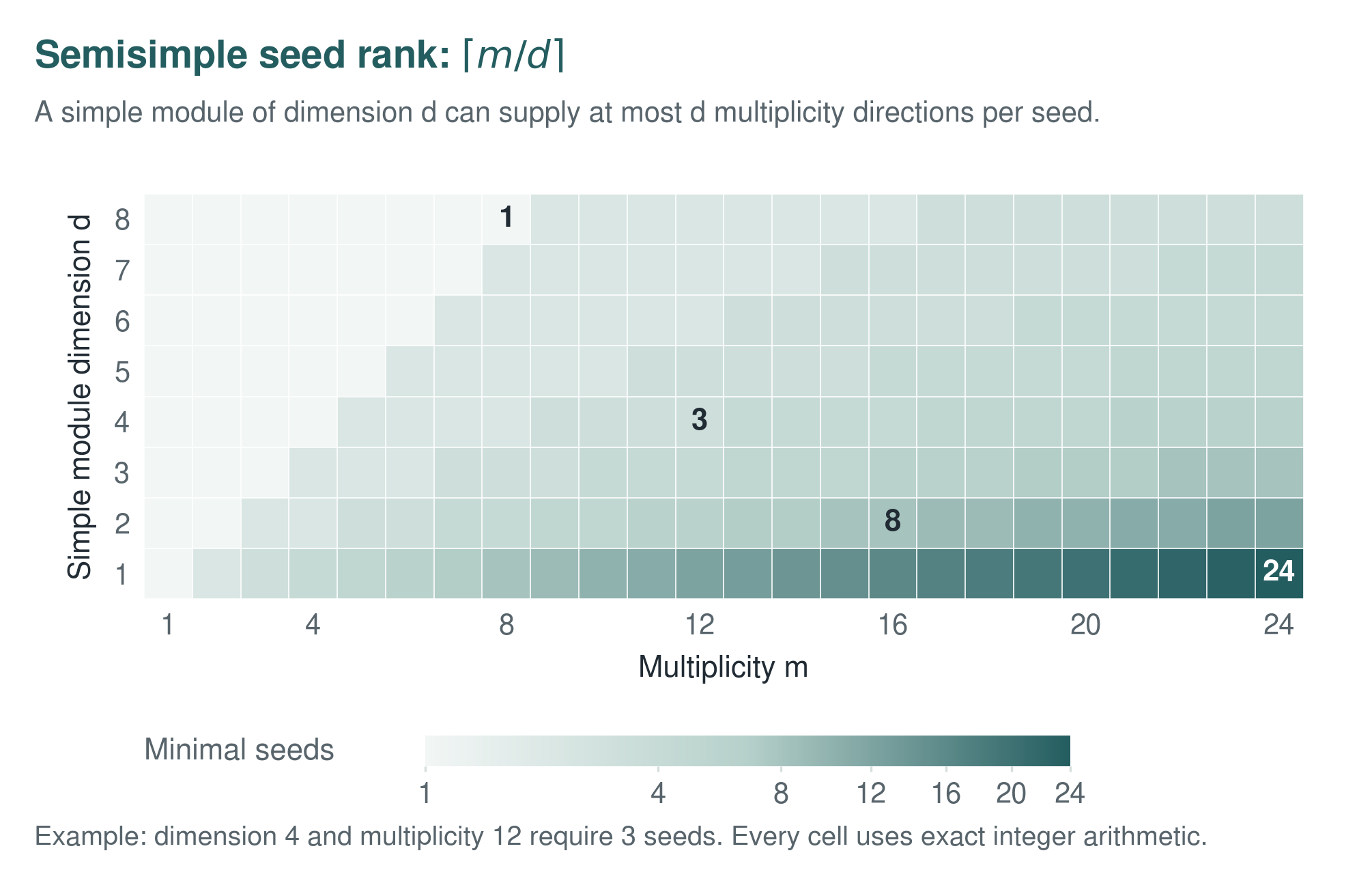
For the factor \(M_{d_i}(D_i)\), one free generator contributes \(d_i\) copies of the corresponding simple module. If the top of \(M\) contains \(m_i\) copies, at least \(\lceil m_i/d_i\rceil\) free generators are required. The worst simple type controls the global answer.
This count concerns copies of a simple module, rather than the number of coordinates in a chosen basis. A single seed can reach several copies through the matrix action. The regular module records precisely how many copies one free generator can supply.
Multiplicity consumes seed capacity
For \(A=M_2({\Bbbk})\) acting on \(({\Bbbk}^2)^{\oplus3}\), the regular module contributes two copies of the natural simple module per generator. One generator cannot cover all three multiplicity directions. Two can, giving seed rank \(2\).
Corollary 5.7: Algebraically closed multiplicity formula
Let \({\Bbbk}\) be algebraically closed, let \(A\) be a unital algebra of finite dimension over \({\Bbbk}\), put \(J={\operatorname{Jac}}(A)\), and let \(M\) be a finitely generated left module over \(A\). Assume compatible decompositions indexed by an integer \(q\geq0\):
where the \(d_i\) are positive integers and the \(m_i\) are nonnegative integers. The first isomorphism is an isomorphism of algebras over \({\Bbbk}\). The second is an isomorphism of left modules over \(A/J\), using the natural column module for each matrix factor and zero action from the other factors. Then
with \(\max\varnothing=0\) when \(q=0\).
Read proof · Visual guide: How much row space can one seed supply? · Read statement and proof side by side · Permalink · Source line 809 · Claim record · Lean coverage · Code · Worked examples
Proof of Corollary 5.7
By Theorem 5.2, \({\operatorname{srank}}_A(M)={\operatorname{srank}}_{A/J}(M/JM)\). Apply Theorem 5.6 to the displayed decompositions of \(A/J\) and \(M/JM\), with every \(D_i={\Bbbk}\). This gives the stated maximum. If \(q=0\), the unital \(A/J\)-module \(M/JM\) is zero, and Theorem 5.2 gives seed rank zero.
Back to statement · Read statement and proof side by side · Permalink · Source line 826 · Claim record · Lean coverage · Code · Worked examples
Corollary 5.8: Full matrix algebra
For the natural module \(S=D^d\) over \(M_d(D)\),
More strongly, every nonzero vector of \(S\) is cyclic.
Read proof · Read statement and proof side by side · Permalink · Source line 830 · Claim record · Lean coverage · Code · Worked examples
Proof of Corollary 5.8
The formula gives \(\lceil1/d\rceil=1\). Directly, let \(v\neq0\) and choose a coordinate \(v_j\neq0\). For any target \(w=(w_i)\), the matrix whose \(j\)th column has entries \(w_iv_j^{-1}\) and whose other columns vanish sends \(v\) to \(w\).
Back to statement · Read statement and proof side by side · Permalink · Source line 841 · Claim record · Lean coverage · Code · Worked examples
Corollary 5.9: Multiplicity obstruction
For the diagonal action of \(M_d(D)\) on \(S^{\oplus m}\),
Read proof · Read statement and proof side by side · Permalink · Source line 845 · Claim record · Lean coverage · Code · Worked examples
Proof of Corollary 5.9
Apply Theorem 5.6 to the single simple type with multiplicity \(m\).
Back to statement · Read statement and proof side by side · Permalink · Source line 859 · Claim record · Lean coverage · Code · Worked examples
Section recap
For finitely generated modules, the minimal number of seeds is detected on the quotient by the Jacobson radical. In the semisimple top, each generator has a fixed multiplicity capacity \(d_i\) in simple type \(i\), and the largest capacity ratio determines the exact seed rank.
6 Modules for a single operator over arbitrary fields
On this page · Permalink · Source line 874
Reader roadmap
One operator is equivalent to a module over \({\Bbbk}[t]\). Primary decomposition isolates the irreducible polynomial sectors, and the quotient by \(p(T)\) counts how many cyclic chains begin in each sector.
6.1 Primary components and generator counts
On this page · Permalink · Source line 881
Classical input 6.1: Primary decomposition for polynomial modules
Every module \(X\) over \({\Bbbk}[t]\) with finite dimension over the coefficient field decomposes as
where \({\operatorname{Irr}}({\Bbbk}[t])\) denotes the monic irreducible polynomials, only finitely many components are nonzero, and every nonzero \(X_p\) is a finite direct sum of modules \({\Bbbk}[t]/(p^e)\).
Permalink · Source line 883 · Claim record · Lean coverage · Code · Worked examples
Theorem 6.2: Seed rank for a single operator
Let \(X\) have finite dimension over \({\Bbbk}\) and let \(T\in{\operatorname{End}}_{{\Bbbk}}(X)\). Regard \(X\) as a module over \({\Bbbk}[t]\) by \(t\cdot x=Tx\). For every monic irreducible \(p\), let \(X_p\) be the primary component for \(p\) and set
Then
Moreover, \(\mu_p(T)\) is the number of cyclic primary summands for \(p\) in the decomposition into elementary divisors of \(X_p\).
Read proof · Visual guide: Two chains can stay linked · Visual guide: A quotient proves two seeds are necessary · Visual guide: Distinct labels let one polynomial separate chains · Read statement and proof side by side · Permalink · Source line 893 · Claim record · Lean coverage · Code · Worked examples
Proof of Theorem 6.2
Let the minimal polynomial be
The acting algebra is
by the Chinese remainder theorem. The factor \(R_p\) acts on \(X_p\) and annihilates every other primary component. Hence the formula for a direct sum with independent actions gives
Each \(R_p\) is local with maximal ideal generated by the class of \(p\) and residue division field \(K_p={\Bbbk}[t]/(p)\). By Corollary 5.3,
Finally, every summand \({\Bbbk}[t]/(p^e)\) contributes one copy of \(K_p\) after quotienting by \(p\), so the dimension equals the number of summands in the elementary divisor decomposition.
Back to statement · Read statement and proof side by side · Permalink · Source line 914 · Claim record · Lean coverage · Code · Worked examples
How to read the result
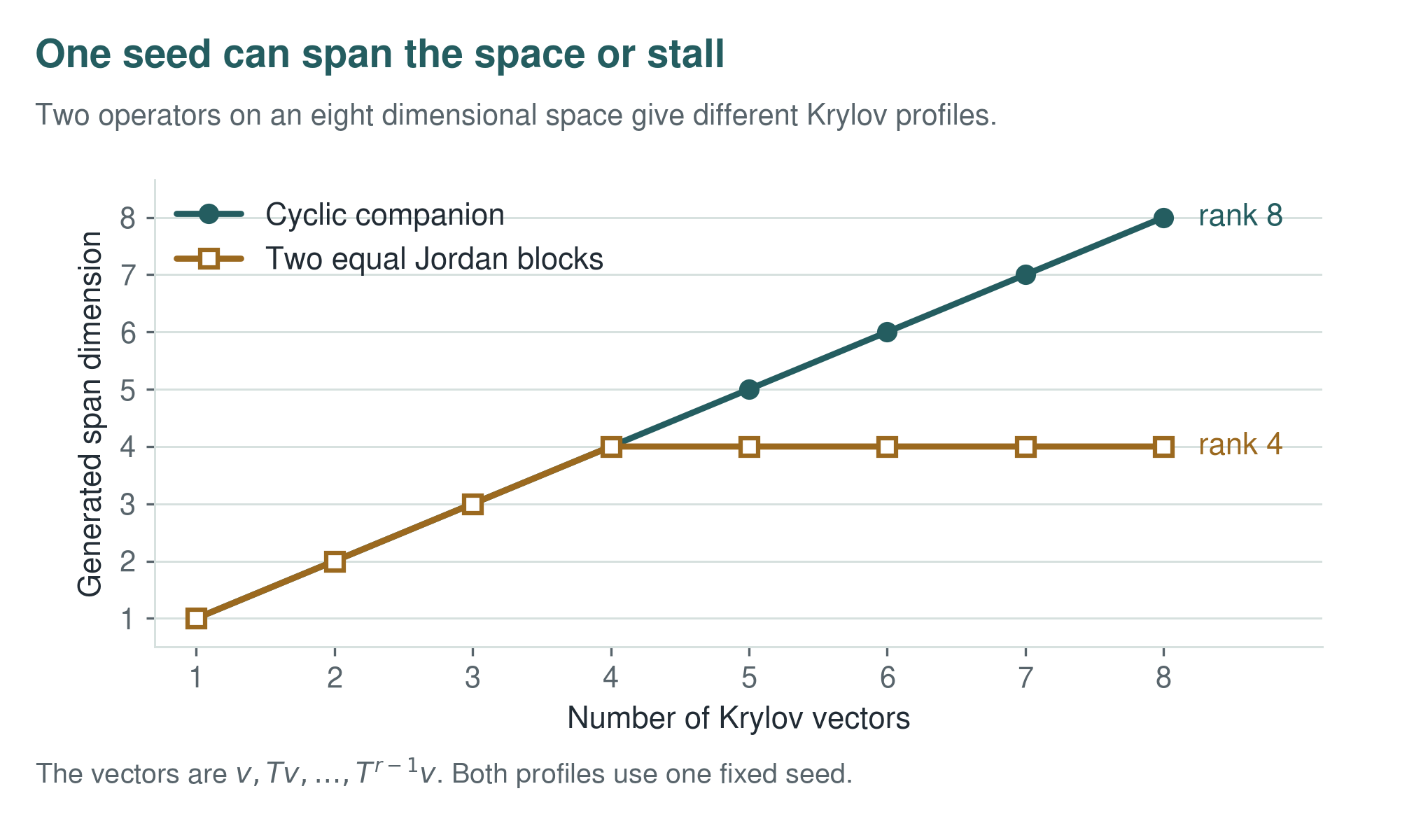
For one operator, the quotient \(X_p/p(T)X_p\) counts the number of independent primary chains for the irreducible polynomial \(p\). Over an algebraic closure these become Jordan chains. The seed rank is the largest chain count among the primary sectors, not the largest chain length.
Block count versus block size
A nilpotent operator with Jordan block sizes \((5,1,1)\) has seed rank \(3\), even though its largest block has length \(5\). Three seeds are needed because there are three independent chains. Once their initial vectors are chosen, repeated application of \(T\) generates every position in those chains.
6.2 Invariant factors, Jordan blocks, and cyclicity
On this page · Permalink · Source line 950
Corollary 6.3: Invariant factor count
If \(X\neq0\) and the rational canonical decomposition is written with nonconstant invariant factors
then
Read proof · Visual guide: Distinct labels let one polynomial separate chains · Read statement and proof side by side · Permalink · Source line 951 · Claim record · Lean coverage · Code · Worked examples
Proof of Corollary 6.3
For each irreducible \(p\), the number of invariant factors divisible by \(p\) equals the number of elementary divisors for \(p\). Because \(f_1\mid\cdots\mid f_r\) and \(f_1\neq1\) after zero summands are removed, some irreducible divisor of \(f_1\) divides all \(r\) invariant factors. Hence \(\max_p\mu_p(T)=r\).
Back to statement · Read statement and proof side by side · Permalink · Source line 967 · Claim record · Lean coverage · Code · Worked examples
Corollary 6.4: Formula for geometric multiplicity
If \({\Bbbk}\) is algebraically closed, then
Read proof · Read statement and proof side by side · Permalink · Source line 971 · Claim record · Lean coverage · Code · Worked examples
Proof of Corollary 6.4
The irreducibles are \(p=t-\lambda\). On the primary component for \(\lambda\), the quotient by \((T-\lambda I)X_\lambda\) has dimension equal to the number of Jordan blocks, which is also \(\dim{\operatorname{Ker}}(T-\lambda I)\).
Back to statement · Read statement and proof side by side · Permalink · Source line 986 · Claim record · Lean coverage · Code · Worked examples
Corollary 6.5: Criterion for a cyclic matrix
For \(X\ne0\) of finite dimension, the following are equivalent:
\(T\) has a cyclic vector.
\({\operatorname{srank}}_{{\Bbbk}[T]}(X)=1\).
Every nonzero primary component for \(p\) is cyclic.
The rational canonical form has one invariant factor.
The minimal polynomial equals the characteristic polynomial.
After scalar extension to an algebraic closure, every eigenvalue has geometric multiplicity one.
Read proof · Read statement and proof side by side · Permalink · Source line 990 · Claim record · Lean coverage · Code · Worked examples
Proof of Corollary 6.5
The equivalence of (i) and (ii) is Proposition 4.2. By Theorem 6.2, (ii) holds exactly when every \(\mu_p(T)\) belonging to a nonzero primary component equals one, which is (iii). Relatively prime primary cyclic modules combine into one cyclic module by the Chinese remainder theorem, so (iii) is equivalent to (iv). In rational canonical form, one invariant factor means that the unique invariant factor is both the minimal and characteristic polynomial, proving (iv)\(\Leftrightarrow\)(v). Scalar extension preserves the equality of minimal and characteristic polynomials. Over an algebraic closure, that equality is equivalent to one Jordan block for each eigenvalue, which is (vi).
Back to statement · Read statement and proof side by side · Permalink · Source line 1005 · Claim record · Lean coverage · Code · Worked examples
Section recap
A single operator is cyclic exactly when each primary sector has one cyclic chain. Over an algebraic closure this is equivalent to one Jordan block per eigenvalue and to equality of the minimal and characteristic polynomials.