
13 A typed quiver model
On this page · Permalink · Source line 1
A small quiver model shows how the path algebra records a direction that the available seeds cannot reach.
Let the quiver have vertices \(U,V\) and arrows
with the relation in the path algebra
whose realization is the operator identity \(BA=I_U\). Realize
by
Starting from the seed \(e_1\in U\), repeated application of \(R\) spans \(U\), and \(A\) carries that span onto the first two coordinates of \(V\). Any path from \(U\) to \(V\) ends with \(A\) and therefore lands in \({\operatorname{im}} A\). The third coordinate direction, which spans \(\ker B\), is unreachable from a seed supported only at \(U\). Therefore the generated representation is
Adding the seed \((0,0,1)\in V\) generates the full representation.
Proposition 13.1: Typed reachability certificate
In the preceding quiver realization, no seed supported at \(U\) can generate the full representation, whereas the two seeds
do generate it.
Visual guide: A reached type can still hide a direction · Permalink · Source line 40
Proof
The first claim follows because every path that starts at \(U\) and ends in \(V\) has final arrow \(A\), so its image lies in \({\operatorname{im}} A\). For the second, \(e_1\) and \(Re_1\) span \(U\). Their images under \(A\) span \({\operatorname{im}} A\), and \(e_3\) spans \(\ker B\), the missing complementary direction in \(V\).
This example shows why a typed grammar is more than a notational convenience. The obstruction lies in the subspace \(\ker B\subset V\), which is unreachable from seeds supported at \(U\), and is visible before any coordinate calculation.
The arrow from one vertex to another records which type can be reached. Its image records which directions can be reached within that type. Here the first seed reaches both vertices, yet misses one direction at the second vertex. The extra seed supplies that direction directly. This is why reachability of a vertex alone does not settle generation of its entire space.
14 Worked algebraic model: an elliptic coordinate ring
On this page · Visual guide: A relation becomes a packet product rule · Permalink · Source line 59
Let \(\operatorname{char}{\Bbbk}\ne2\) and let
The affine equation \(y^2=x^3-x\) has classical discriminant \(64\), which is nonzero under this hypothesis. Standard algebraic geometry then identifies its smooth projective completion as an elliptic curve [silverman2009]. The Lean development checks the algebraic implication \(2\ne0\Rightarrow64\ne0\), the quotient normal form, and the operator identities below. It does not formalize projective smoothness, genus, or the geometric identification of the discriminant. The packet computation itself uses only the displayed relation in the quotient ring. Every class has a unique normal form
Indeed, \(y^2-(x^3-x)\) is monic of degree two in \(y\), so division in \({\Bbbk}[x][y]\) gives a unique remainder of degree less than two in \(y\). Concretely, every power \(y^m\) with \(m\ge2\) can be reduced using
14.1 One module seed and two address operators
On this page · Permalink · Source line 75
Take the seed
and let \(M_x,M_y\) be multiplication by \(x\) and \(y\). Then
so the algebra, regarded as a module over its multiplication algebra, is generated by one seed.
The two packet spaces are
Let
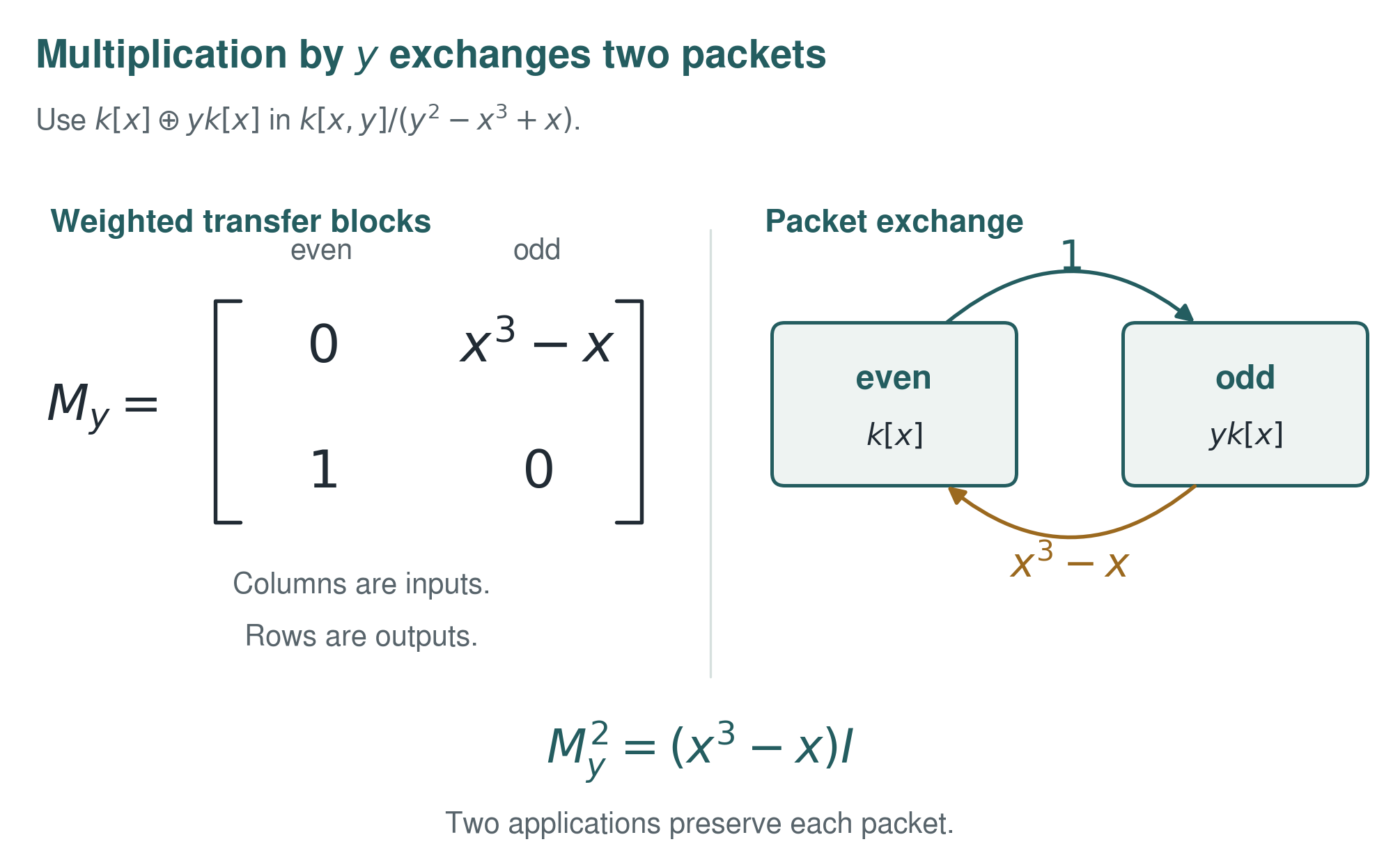
These idempotents are linear over \({\Bbbk}\), annihilate one another, and satisfy \(P_0+P_1=I\). They are not module maps over \(A\), because multiplication by \(y\) exchanges the two packets.
Identify the packet coefficients by
In these ordered coefficient coordinates, with \(M_x\) and \(M_{x^3-x}\) denoting multiplication on \({\Bbbk}[x]\),
The two rows of the second matrix record the outgoing packet coefficients. An even input enters the odd packet without an additional factor. An odd input returns to the even packet through the factor imposed by the curve equation. Applying the matrix twice therefore preserves each packet and multiplies its coefficient by that factor.
The relation is reconstructed as an operator identity:
14.2 Exact product law
On this page · Visual guide: A relation becomes a packet product rule · Permalink · Source line 137
Write
Then
This is a convolution law for the two packets. It is already visible at the linear operator level because multiplication by a fixed element is a transfer operator. The even output collects the product of the two even coefficients and the weighted product of the two odd coefficients. The odd output collects the two products with one even and one odd coefficient. The quotient relation is thus retained in the weight rather than discarded during the decomposition.
Example 14.1: Worked reduction
Take
Then
Thus
The symbolic certificate in the companion code performs the same quotient reduction exactly.
14.3 What this example establishes
On this page · Permalink · Source line 182
The coordinate ring illustrates four distinct parts of the calculus:
the unit is a module seed.
\(M_x\) and \(M_y\) are address operators.
the curve equation is an operator relation.
parity in \(y\) gives exact packet analysis, transfer, and reconstruction.
It does not imply that every algebra can be presented as an algebra generated by one element. It shows instead that unital algebras are cyclic as modules over their full multiplication algebra.
15 Worked signal model: a bilateral shift
On this page · Permalink · Source line 193
Let \(\mathbb{F}\in\{{\mathbb R},{\mathbb C}\}\) and let
with a family of bounded reindexing operators indexed by the integers
Thus \(S_0=I\), \(S_{m+r}=S_mS_r\), and \(S_1\) is the usual bilateral shift. We use the standard conventions for Hilbert spaces and bounded operators of [conway1990]. The impulse \(\delta_0\) satisfies
for every \(m\in{\mathbb Z}\). Therefore sequences with finite support lie in its algebraic orbit hull and are dense in \(\ell^2({\mathbb Z})\).
Proposition 15.1: Shift seed
For \(n\in{\mathbb N}\), let \(G(n)\) mean that some finite seed set with \(n\) elements has dense hull under the declared family \(\{S_m:m\in{\mathbb Z}\}\). Then
Equivalently, one seed suffices and no empty seed family generates densely.
Visual guide: Density is not finite generation of each vector · Permalink · Source line 211
Proof
The orbit of \(\delta_0\) contains every standard basis vector. Their finite linear span is dense, so \(G(1)\) holds. The hull of the empty seed set is zero, while \(\ell^2({\mathbb Z};\mathbb F)\) is nonzero, so \(G(0)\) fails. Therefore \(1\) is the least admissible finite cardinality.
For \(N\ge1\), define residue projectors
They form an orthogonal packet system and satisfy
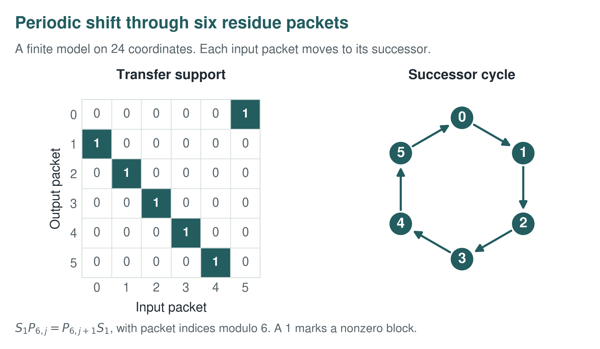
with indices modulo \(N\). The shift is therefore a cyclic transfer between residue packets.
The seed claim concerns density, rather than equality with the algebraic hull. Finite linear combinations of shifted impulses give precisely the sequences with finite support. Taking their closure gives the whole Hilbert space. The packet decomposition and the choice of completion answer different questions, and both must be specified for this realization.
Boundary 15.2
This section uses residue packets only to demonstrate the foundational transfer algebra. Nested refinement and structures for filter banks require additional definitions and are outside Paper I.
16 Worked matrix models
On this page · Permalink · Source line 252
16.1 The full matrix algebra
On this page · Permalink · Source line 254
Let \(X={\Bbbk}^n\) and let \({\mathcal A}=M_n({\Bbbk})={\operatorname{End}}_{{\Bbbk}}(X)\), with the full matrix algebra declared before a seed or target is chosen. By Corollary 5.8, every nonzero seed is cyclic. This is the maximal linear grammar on \(X\). It does not give a compression result. Under a smaller declared operator algebra, the same vector need not be cyclic.
16.2 Companion operators and repeated blocks
On this page · Permalink · Source line 258
For one operator \(T\), Theorem 6.2 turns verified primary data into an exact certificate for the minimum number of seeds. The numerical companion compares:
a nilpotent companion operator with one Jordan chain, for which the Krylov rank is \(1,2,\ldots,n\).
two equal Jordan blocks, for which one diagonal seed produces a chain only as long as one block and then stalls.
The observed stall is not numerical failure. The associated scalar quotient of dimension two certifies the lower bound in Theorem 6.2. Identifying that quotient with the space that measures geometric multiplicity is the classical Jordan input stated above.
17 Worked graph model: adjacency algebras
On this page · Permalink · Source line 272
Let \(G\) be a nonempty finite graph with adjacency matrix \(A_G\), and regard \({\Bbbk}^{V(G)}\) as a module over \({\Bbbk}[A_G]\). The general result applies directly to a spectral certificate. For a symmetric real adjacency matrix, the classical spectral theorem supplies such data.
Within one eigenspace, every polynomial in the adjacency operator acts by a scalar. A seed therefore supplies at most one vector direction in that eigenspace. Distinct eigenvalues can be separated by projector polynomials, so the same seed may supply one direction to each of several eigenspaces. With a complete eigenbasis, the largest eigenspace determines how many seeds are needed, rather than the number of distinct eigenvalues.
Corollary 17.1: Certified graph seed number
Let \({\Bbbk}\) be a field and let \(\Lambda\) be a nonempty finite set. Suppose there are pairwise distinct scalars \(a_{\lambda}\in{\Bbbk}\), multiplicities \(m_{\lambda}\in{\mathbb N}\), and an eigenbasis
of \({\Bbbk}^{V(G)}\) satisfying
If \(m_{\lambda}\le R\) for all \(\lambda\) and \(m_{\lambda_*}=R\) for some \(\lambda_*\), then \(R\) is the least natural number of adjacency seeds:
Proof
The distinct eigenvalue labels give Lagrange polynomials that project onto the individual eigenspace packets. Padding one basis vector from every packet into each of \(R\) seeds gives the upper bound. Projection to the \(m_{\lambda}\) eigenspace coordinates is a surjective scalar quotient, so any generating family has at least \(m_{\lambda}\) members for every \(\lambda\). The label \(\lambda_*\) gives the matching lower bound \(R\).
Boundary 17.2: Input from spectral classification
For a finite undirected graph over \({\mathbb C}\), the spectral theorem for real symmetric matrices classically supplies a certificate of the displayed kind, and the numbers \(m_{\lambda}\) are the usual eigenvalue multiplicities. See [brouwerHaemers2012]. The formal declaration verifies the formula for the number of seeds from the supplied eigenbasis and distinct eigenvalue labels. It does not derive diagonalizability from symmetry or implement an eigensolver.
17.1 Path graphs
On this page · Visual guide: Walk counts make an endpoint cyclic · Permalink · Source line 326
For every field \({\Bbbk}\) and every \(n\ge1\), an endpoint of \(P_n\) is a cyclic vector for the adjacency operator. Consequently one is the least finite number of adjacency seeds:
Over \({\mathbb C}\), the familiar spectral description has the distinct eigenvalues
and the normalized eigenvectors have endpoint coordinate proportional to
There is also a combinatorial proof valid over every field. Let
Its \((i,j)\) entry counts walks of length \(j-1\) from the first vertex to vertex \(i\). This entry is zero when \(i>j\), while the diagonal entry is one because there is a unique shortest walk of length \(i-1\) from vertex \(1\) to vertex \(i\). Hence \(K_n\) is upper triangular with unit diagonal, so
Thus the endpoint is cyclic for every path size, not merely for the tested range.

17.2 Cycle graphs
On this page · Visual guide: Closing a path changes the seed obstruction · Permalink · Source line 366
Two adjacent vertex vectors generate the adjacency module of every simple cycle. Over \({\mathbb C}\), a Fourier quotient built from a primitive root of unity supplies a matching scalar obstruction of dimension two. Hence, for every \(n\ge3\), two is the least finite number of adjacency seeds:
To see the upper bound directly, index the vertices modulo \(n\). The identity \(Ae_j=e_{j-1}+e_{j+1}\) recovers successive vertex vectors from \(e_0\) and \(e_1\), over any field. For the lower bound over \({\mathbb C}\), let \(\zeta\) be a primitive \(n\)th root of unity and define
Then \(q(Ax)=(\zeta+\zeta^{-1})q(x)\). The images of \(e_0\) and \(e_1\) are \((1,1)\) and \((\zeta,\zeta^{-1})\), which are independent because \(\zeta\ne\zeta^{-1}\) for \(n\ge3\). Thus \(q\) is a scalar quotient of dimension two, and Proposition 4.13 gives the matching lower bound.
The usual spectral description writes the eigenvalues as
The values for \(k\) and \(n-k\) coincide. Apart from the simple characters at \(k=0\) and, for even \(n\), \(k=n/2\), the remaining Fourier characters occur in pairs. Therefore the maximum eigenspace multiplicity is two, although some eigenspaces have multiplicity one, and the certified minimum above is two.

The path and cycle examples use nearly identical local operators. Their minimum finite seed numbers differ because the path has an endpoint Krylov basis, whereas the cycle has a Fourier quotient obstruction of dimension two.
18 The common operator language
On this page · Permalink · Source line 414
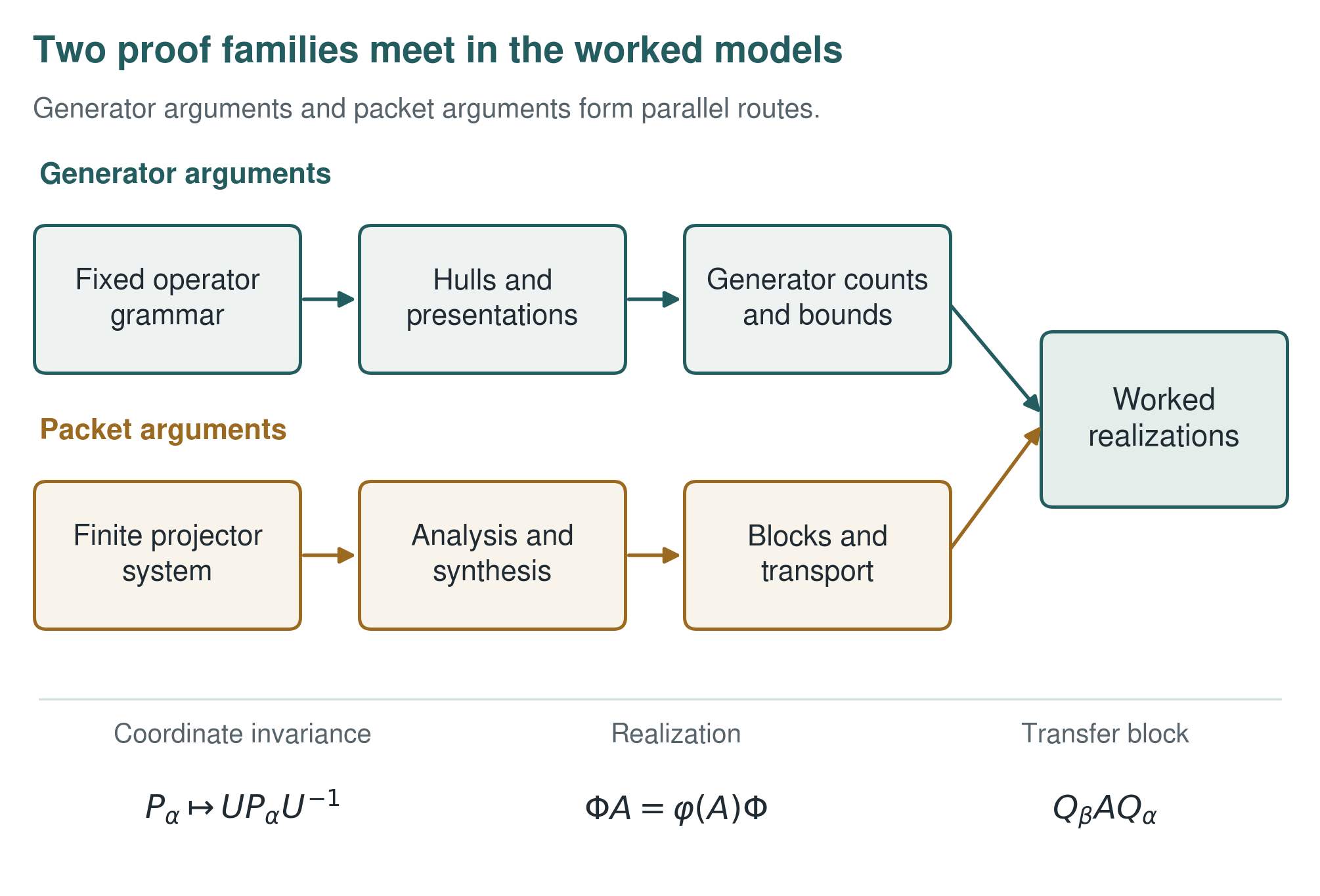
The preceding examples can be written without changing the foundational notation.
| Realization | Seed | Operator grammar | Packets | Completion or quotient |
|---|---|---|---|---|
| Coordinate ring | \(1\) | \(M_x,M_y\) | even/odd \(y\) degree | quotient by \(y^2-x^3+x\) |
| Shift system | \(\delta_0\) | \((S_m)_{m\in{\mathbb Z}}\) | residue classes of \(n\) | \(\ell^2\) closure |
| Full matrix module | \(s\ne0\) | \(M_n({\Bbbk})\) | chosen idempotents | finite dimensional |
| Single operator | \(s_1,\ldots,s_r\) | \({\Bbbk}[T]\) | primary or spectral | finite dimensional |
| Graph adjacency | vertex seeds | \({\Bbbk}[A_G]\) | eigenspaces | finite dimensional |
| Typed grammar | vertex seeds | path algebra \({\Bbbk} Q/I\) | vertex idempotents | relation quotient |
For a finite ordered seed family \(S=(s_1,\ldots,s_r)\), let \(\varepsilon_S:{\mathcal A}^{\oplus r}\to X\) be the seed evaluation map of Definition 3.1. Its kernel is the relation module. The free module modulo that kernel presents the generated hull by Theorem 3.2. The invariant content is:
19 Computational certificates
On this page · Permalink · Source line 461
The accompanying Python package is not used as a substitute for proof. It provides exact symbolic checks and finite numerical regression tests for formulas already proved. The computed ranges and random seeds are recorded explicitly. These checks do not extend a theorem beyond its hypotheses or certify an unrestricted numerical implementation. The journal companion also tests integer counts beyond the precision of floating point arithmetic and rejects the unsupported spectral shortcut for complex symmetric matrices.
19.1 Test suite
On this page · Permalink · Source line 465
The test suite checks:
projector idempotence, annihilation, and completeness.
exact vector analysis and synthesis.
exact operator reconstruction from all transfer blocks.
coordinate transport under a dense random similarity transform.
cyclicity of a companion operator.
the obstruction that requires two seeds for repeated Jordan blocks.
the semisimple multiplicity formula in representative cases.
full orbit dimension for two representative nonzero seeds under the full matrix algebra.
exact reduction and packet multiplication in the elliptic coordinate ring.
seed ranks of path and cycle adjacency modules over the reported finite ranges.
the cyclic residue transfer pattern of a finite shift.
19.2 Recorded results
On this page · Permalink · Source line 482
| Quantity | Result |
|---|---|
| Projector idempotence residual | \(0\) |
| Projector annihilation residual | \(0\) |
| Projector completeness residual | \(0\) |
| Operator reconstruction residual | \(0\) |
| Residual for transported projectors, maximum | \(1.85\times10^{-15}\) |
| Companion seed rank | \(1\) |
| Two equal Jordan blocks, seed rank | \(2\) |
| \(M_3({\mathbb C})\) acting on seven copies, seed rank | \(3\) |
| Sampled path graph seed ranks, \(2\le n\le12\) | \(1\) |
| Sampled cycle graph seed ranks, \(3\le n\le12\) | \(2\) |
| Full \(M_4({\mathbb R})\) orbit dimensions for two sampled nonzero seeds | \(4,4\) |
| Automated tests | \(33/33\) passed |
The finite shift pattern recovered by the experiment is
which is the exact packet adjacency of a cyclic transfer among four phases.
19.3 Algorithms
On this page · Permalink · Source line 519
The following finite constructions state mathematical specifications for the companion. Their Lean counterparts and exact scope are listed in the separate guide. They do not assert code extraction or a particular backend's performance.
Construction 19.1: Closure specification for the orbit hull
Let \(V\) have finite dimension, let \((O_i)_{i\in I}\) be a finite operator family, and let \(S\subseteq V\). Define
Then there is an \(n\in{\mathbb N}\) such that
where the right side is the least subspace containing \(S\) and invariant under every \(O_i\). Thus the ascending subspace iteration terminates and its stable value is exactly the finite operator hull.
Each strict enlargement increases dimension, so finite dimension prevents the iteration from continuing indefinitely. Equality at one step means that applying any declared operator keeps every vector in the current subspace. The stable subspace is therefore invariant, while every earlier step belongs to any invariant subspace that contains the seeds.
Visual guide: Stop when the subspace stops growing · Permalink · Source line 523
Construction 19.2: Table specification for transfer blocks
Given finite projector systems \((P_i)_{i\in I}\) and \((Q_j)_{j\in J}\) and a linear map \(T\), form the table
Its assembly reconstructs the input map exactly,
and its reported support relation is exactly \(\{(i,j):B_{ji}\ne0\}\). The latter equality is the specification of the transfer graph output. It does not claim that Lean extracts a routine that decides the edge list for every coefficient field.
Construction 19.3: Exact graph seed rank from a certificate
For a finite square matrix \(A\) over a field \(K\), define the noncomputable exact spectral quantity
with value zero for an empty spectrum. Suppose an exact certificate supplies a finite eigenbasis indexed by labels and multiplicities, the eigenvalue equations, a multiplicity bound attained by one label, projector polynomials that extract the padded eigenbasis generators, coverage of every spectral value by a label, equality of the declared and actual eigenspace dimensions, and membership of the maximizing eigenvalue in the spectrum. Then \(r_{\mathrm{spec}}(A)\) is the least natural number of seeds under polynomial orbits for \(A\).
This is a verified certificate checker/specification. It does not construct the eigenbasis, prove that a symmetric matrix is diagonalizable, or implement an exact eigensolver. The companion Python code performs symbolic computations in the reported finite graph range. The path and cycle results for every size are proved separately above.
20 Reading guide: common confusions and diagnostic questions
On this page · Permalink · Source line 588
20.1 Common confusions
On this page · Permalink · Source line 590
| Do not conflate | Correct distinction |
|---|---|
| Grammar with realized algebra | The grammar may contain relations or words that act as zero. Seed rank depends only on the image action. |
| Seed with basis vector | A seed is a generator under an algebra action. One seed may generate a module with large dimension. |
| Cyclic vector with eigenvector | A cyclic vector must generate the whole module under operator words. It is usually not an eigenvector. |
| Packet with orthogonal subspace | A packet is the range of an idempotent in a complete annihilating family. Orthogonality is optional. |
| Exact reconstruction with good conditioning | Algebraic inverse identities may coexist with large analysis and synthesis norms. |
| Nonzero transfer edge with surjective transfer | A nonzero block can have small rank. Graph reachability alone does not prove generation. |
| Seed rank for single packet seeds with unrestricted seed rank | Seeds supported in several packets may meet several source components simultaneously. |
| Continuous surjection with quotient isomorphism | The target topology must agree with the quotient topology. |
| Repeated notation with semantic realization | A true realization must preserve a declared collection of operations and identities. |
20.2 Diagnostic questions for a new application
On this page · Permalink · Source line 610
Before claiming that a new subject is a realization of Paper I, answer the following.
What is the fixed operator grammar or acting algebra?
What is the concrete realization space or module?
Which seeds are declared before the target is chosen?
Is generation algebraic, topological, probabilistic, or approximate?
What are the idempotent packets, and in what sense do they sum to the identity?
Are the packets finite, countable unconditional, or merely formal?
What are the transfer blocks, and which blocks are known to vanish?
Which morphisms preserve the packet system?
Which quotient, completion, tensor, or limit operations must be preserved?
What exact theorem from Paper I is being specialized, and what new domain theorem remains to be proved?
20.3 Theorem spine at a glance
On this page · Permalink · Source line 625
\( \begin{array}{c} \text{free seed presentation}\\[0.25em] \Downarrow\\[-0.1em] \text{minimal generator number}\\[0.25em] \Downarrow\\[-0.1em] \text{reduction modulo the Jacobson radical}\\[0.25em] \Downarrow\\[-0.1em] \text{semisimple or primary computation} \end{array} \qquad\qquad \begin{array}{c} \text{packet idempotents}\\[0.25em] \Downarrow\\[-0.1em] \text{exact analysis/synthesis}\\[0.25em] \Downarrow\\[-0.1em] \text{transfer block algebra}\\[0.25em] \Downarrow\\[-0.1em] \text{graphs, quotients, and realization} \end{array} \)