Paper X: Seed zeta functions and branching dimensions

6 Seed zeta functions and branching dimensions

On this page · Permalink · Source line 526

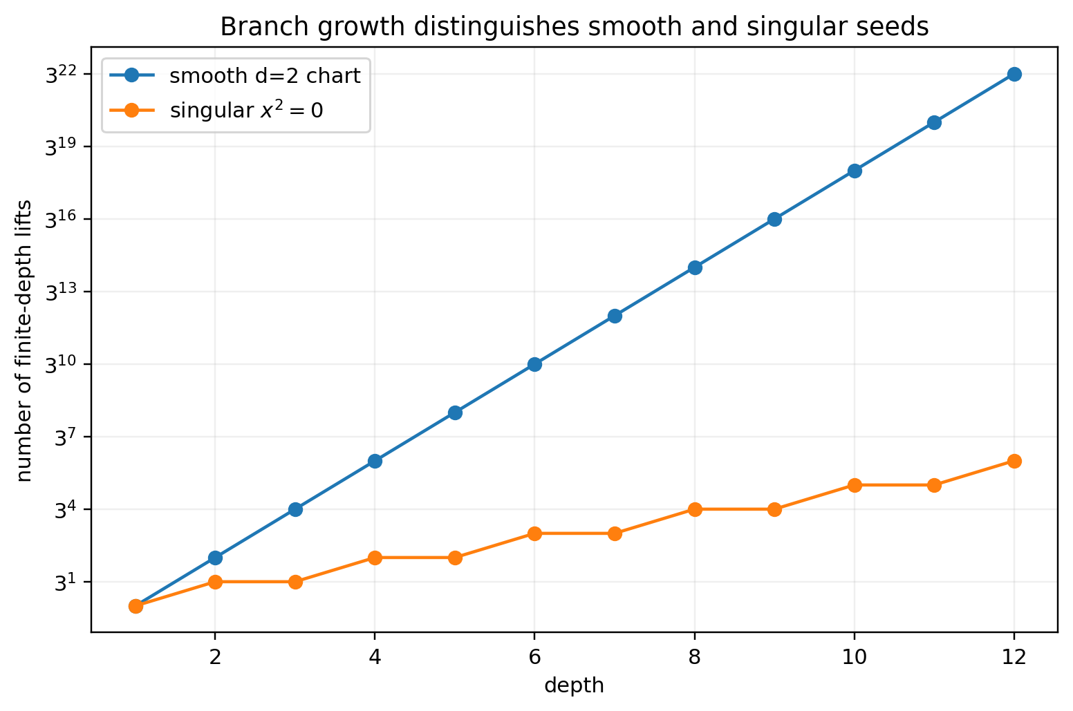
Finite-depth counts record more than the existence of a branch. They distinguish smooth, weighted, and singular local geometry.

Permalink · Source line 528

Definition 6.1: Seed zeta function

For a residual root \(\bar x\) with finite levels, define

\[ \boxed{ Z_{\bar x}(T) = \sum_{m\ge1}\#X_m(\bar x)T^m. } \]

When a weighted chart is specified, write \(Z_{\boldsymbol w}(T)\).

Visual guide: An atlas of the objects · Permalink · Source line 530 · Claim record · Lean coverage · Code · Worked examples

Theorem 6.2: Smooth seed zeta function

For a smooth formal component of dimension \(d\),

\[ \boxed{ Z_d(T)=\frac{T}{1-q^dT}. } \]

Read proof · Visual guide: A smooth chart has independent choices · Read statement and proof side by side · Permalink · Source line 542 · Claim record · Lean coverage · Code · Worked examples

Proof of Theorem 6.2

By the proved formal-model map-to-parameter equivalence, \(\#X_m=q^{d(m-1)}\) counts all the actual local coefficient-algebra maps. Summing the geometric series gives the identity. The checked statement is an equality of infinite formal power series, with zero constant coefficient.

Back to statement · Read statement and proof side by side · Permalink · Source line 551 · Claim record · Lean coverage · Code · Worked examples

Theorem 6.3: Weighted seed zeta function

Let \(1\le w_1\le\cdots\le w_d\), put \(W=\sum_iw_i\), and let

\[ a_m=q^{\sum_i\max(m-w_i,0)}. \]

Then

\[ \boxed{ Z_{\boldsymbol w}(T) = \sum_{m=1}^{w_d}a_mT^m + q^{-W}\frac{(q^dT)^{w_d+1}}{1-q^dT}. } \]

In particular, every weighted smooth chart has a rational seed zeta function.

Read proof · Visual guide: Weights delay visibility · Read statement and proof side by side · Permalink · Source line 555 · Claim record · Lean coverage · Code · Worked examples

Proof of Theorem 6.3

The finite sum records the depths before all coordinates are active. For \(m\ge w_d+1\),

\[ a_m=q^{dm-W}, \]

so the remaining terms form one geometric series.

Back to statement · Read statement and proof side by side · Permalink · Source line 573 · Claim record · Lean coverage · Code · Worked examples

Theorem 6.4: Singular power seed

For integers \(e\ge1\) and \(m\ge1\), in \({\mathcal O}/\varpi^m\) the equation

\[ x^e=0 \]

has exactly

\[ \boxed{ q^{m-\lceil m/e\rceil} } \]

solutions. Its seed zeta function is

\[ \boxed{ Z_e(T) = \frac{\sum_{r=1}^{e}q^{r-1}T^r} {1-q^{e-1}T^e}. } \]

Read proof · Visual guide: Many approximate roots, one limit · Read statement and proof side by side · Permalink · Source line 581 · Claim record · Lean coverage · Code · Worked examples

Proof of Theorem 6.4

The congruence is equivalent to

\[ e\,v_\varpi(x)\ge m, \]

so \(x\) must lie in \(\varpi^{\lceil m/e\rceil}{\mathcal O}/\varpi^m\), which has the stated cardinality. Write \(m=ek+r\), \(1\le r\le e\). The exponent becomes \((e-1)k+r-1\). Summing over \(k\ge0\) and \(1\le r\le e\) gives the rational expression.

Back to statement · Read statement and proof side by side · Permalink · Source line 603 · Claim record · Lean coverage · Code · Worked examples

Definition 6.5: Branching dimension

When the limit exists, define the finite-level counting exponent

\[ \dim_{\mathrm{seed}}(\bar x) = \lim_{m\to\infty} \frac{\log_q\#X_m(\bar x)}{m}. \]

A limsup may be used in general.

Permalink · Source line 611 · Claim record · Lean coverage · Code · Worked examples

Corollary 6.6: Fractional singular dimension

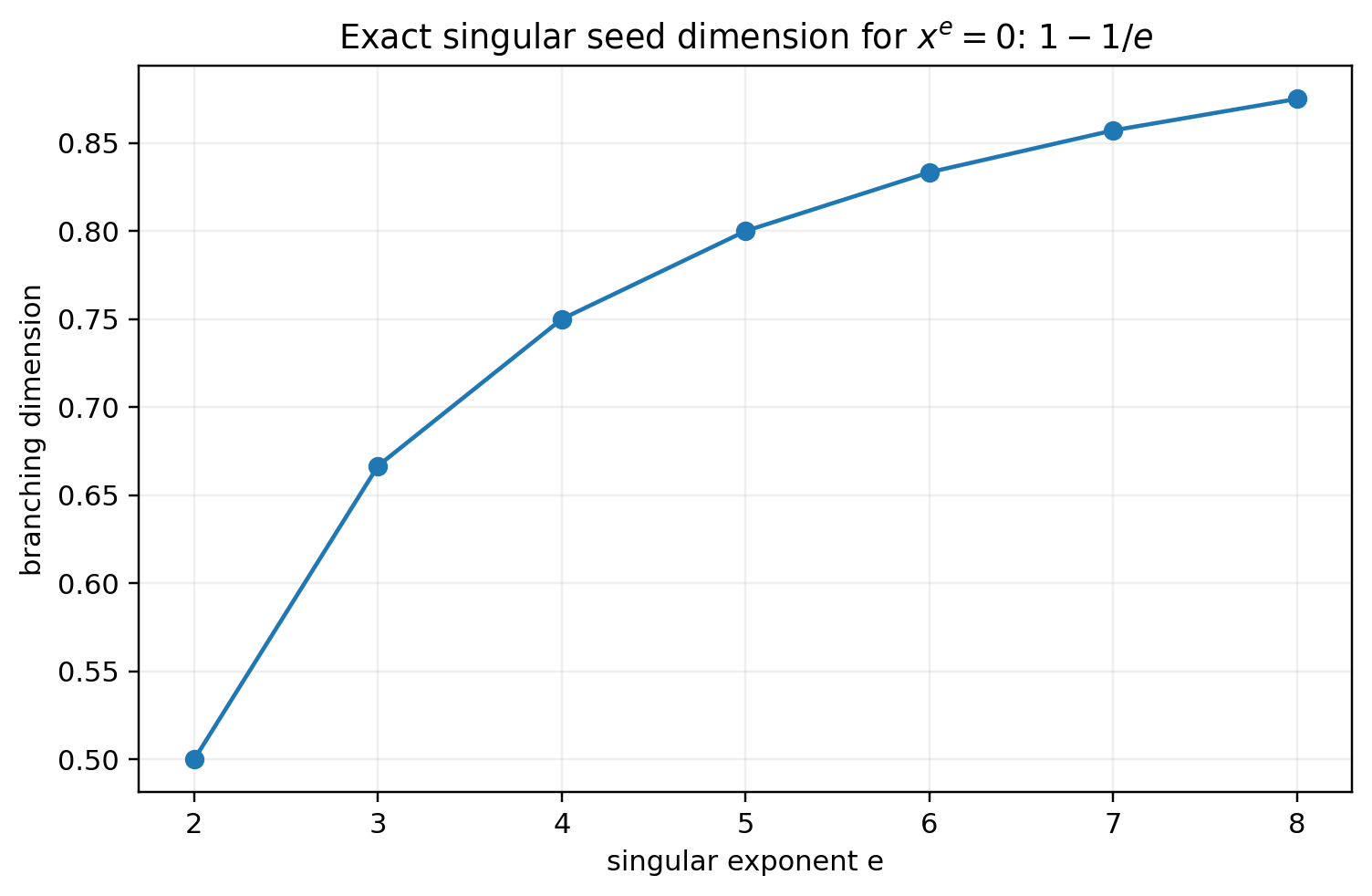
For \(x^e=0\),

\[ \boxed{ \dim_{\mathrm{seed}}=1-\frac1e. } \]

In particular, \(x^2=0\) has branching dimension \(1/2\).

Counting exponent versus compatible branches.

The preceding exponent counts all finite-level solutions, including nodes which cannot lift indefinitely. It is not the cardinality or dimension of the space of infinite branches. In fact every compatible tower of solutions to \(x^e=0\), for \(e\ge1\), is the zero tower. For each \(m\), a solution at depth \(em\) lies in \(\varpi^m{\mathcal O}/\varpi^{em}\); its reduction at depth \(m\) is therefore zero. Compatibility proves the assertion at every depth. This observation and the real logarithmic limit are both formalized in Block 02.

Visual guide: Many approximate roots, one limit · Permalink · Source line 622 · Claim record · Lean coverage · Code · Worked examples

A smooth two-dimensional formal chart and the singular equation (x 2=0 ) have visibly different exponential growth. — A smooth two-dimensional formal chart and the singular equation \(x^2=0\) have visibly different exponential growth.

The finite-depth branching dimension of (x e=0 ) is (1-1/e ), giving a family of fractional local growth exponents. — The finite-depth branching dimension of \(x^e=0\) is \(1-1/e\), giving a family of fractional local growth exponents.

Read and explore

Proofs and implementation

About this work

Other resources