5 The weighted dyadic residual forest
On this page · Permalink · Source line 467
At an odd prime, distinct sign characters remain distinct in the residue field. At the coefficient prime two,
Thus distinct characteristic-zero packets can share one residual root and separate only after more precision is retained.
Definition 5.1: Visibility weight
For two integral packet coordinates \(a,b\in{\mathcal O}\), define their separation depth
when such an \(m\) exists. A dyadic packet decomposition is weighted by these first visibility depths and by the valuations of any denominators required by its rational projectors.
Visual guide: An atlas of the objects · Permalink · Source line 475 · Claim record · Lean coverage · Code · Worked examples
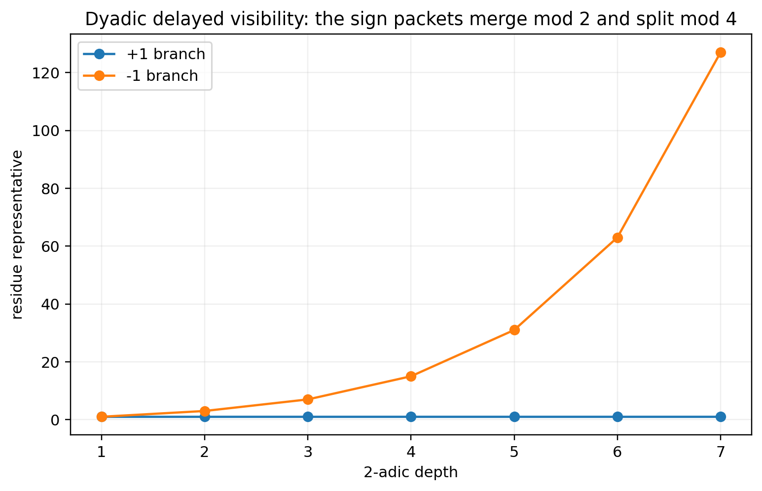
Example 5.2: The two sign branches
The characters \(\chi_+(g)=1\) and \(\chi_-(g)=-1\) have the same reduction modulo \(2\), but
Their first separation depth is therefore \(2\). One mod-two root contains two branches that become distinct at the next level.
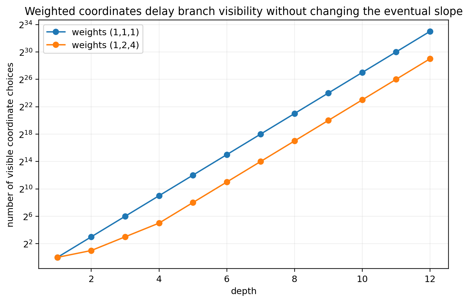
A simple weighted formal model already captures delayed visibility. Let \(w_i\ge1\) and constrain
Then coordinate \(i\) is invisible until \(m>w_i\).
Proposition 5.3: Weighted smooth-chart count
For weights \(\boldsymbol w=(w_1,\ldots,w_d)\),
Read proof · Visual guide: Weights delay visibility · Read statement and proof side by side · Permalink · Source line 503 · Claim record · Lean coverage · Code · Worked examples
Proof of Proposition 5.3
The image of \(\varpi^{w_i}{\mathcal O}\) in \({\mathcal O}/\varpi^m\) has one element when \(m\le w_i\), and \(q^{m-w_i}\) elements when \(m>w_i\). Multiplying the independent coordinate counts gives the formula.
Back to statement · Read statement and proof side by side · Permalink · Source line 514 · Claim record · Lean coverage · Code · Worked examples
This model does not assert that every dyadic Galois deformation ring is a weighted formal ball. It gives the exact local counting law once such weighted coordinates or a Smith-normal-form chart have been proved.