I.1 The quantum seed realization
On this page · Permalink · Source line 1
Conventions.
On this page · Permalink · Source line 3
Unless the zero space is explicitly included as a boundary case, quantum state spaces are nonzero complex Hilbert spaces of finite dimension. A complete packet family is a finite collection satisfying
\[
P_\alpha^*=P_\alpha,\qquad
P_\alpha P_\beta=\delta_{\alpha\beta}P_\alpha,\qquad
\sum_\alpha P_\alpha=I.
\]
All operator norms in the analytic estimates are induced by the norm on the Hilbert space. The estimates do not use the entrywise maximum norm or the Frobenius norm. We write \([A,B]=AB-BA\) and use units with \(\hbar=1\). Parameter derivatives are real derivatives. A matrix \(X\) is supported on a code projector \(P\) when \(PXP=X\).
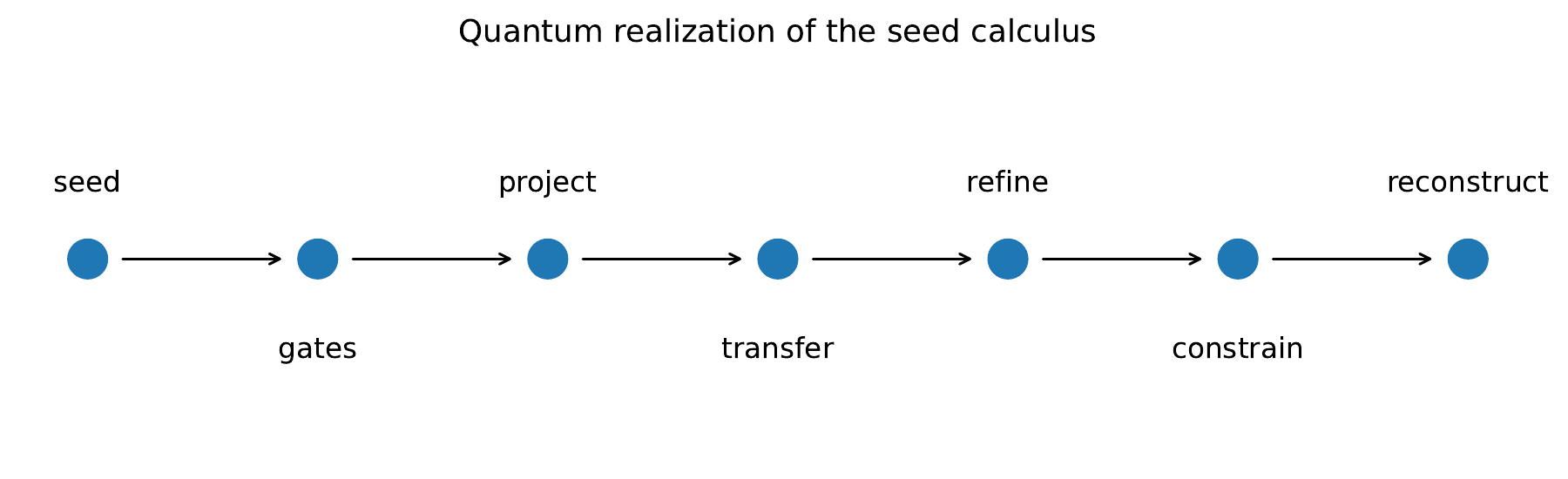
The common operator sequence of the series becomes
\[
\boxed{
\begin{gathered}
\text{quantum seed}
\longrightarrow
\text{gate or observable address}
\longrightarrow
\text{symmetry projection}\\
\longrightarrow
\text{packet transfer}
\longrightarrow
\text{constraint}
\longrightarrow
\text{refinement}
\longrightarrow
\text{reconstruction}
\end{gathered}
}
\]
Permalink · Source line 4
Definition I.1.1: Finite quantum seed system
A finite quantum seed system is a tuple
\[
\mathfrak Q=
\left(
{\mathcal H},
\psi_0,
{\mathcal O},
{\mathcal R},
\{P_{\ell,\alpha}\},
H,
\tau
\right),
\]
where \({\mathcal H}\) is a finite-dimensional Hilbert space, \(\psi_0\in{\mathcal H}\) is a nonzero seed, \({\mathcal O}\) is the declared operator grammar, \({\mathcal R}\) is a collection of algebraic or physical constraints, \(\{P_{\ell,\alpha}\}\) is an exact packet system at each refinement level, \(H=H^*\) is a Hamiltonian when dynamics are present, and \(\tau\) specifies the topology used in a later completion.
Permalink · Source line 40 · Claim record · Lean coverage · Code · Worked examples
The generated state space is
\[
{\mathcal H}(\psi_0;{\mathcal O})
=
\operatorname{span}
\left\{
O_r\cdots O_1\psi_0:
O_j\in{\mathcal O},
\ r\ge0
\right\}.
\]
The quantum seed is cyclic for the grammar when
\[
{\mathcal H}(\psi_0;{\mathcal O})={\mathcal H}.
\]
This is a statement about the pair \((\psi_0,{\mathcal O})\), not about the vector alone. A state may be cyclic for the full matrix algebra and noncyclic for a restricted physical gate set.
Permalink · Source line 57
I.2 Quantum seed rank and cyclicity
On this page · Permalink · Source line 74
I.2.1 Finite observable algebras
On this page · Permalink · Source line 76
Let a finite-dimensional unital \(*\)-subalgebra of operators act in its standard multiplicity form
\[
{\mathcal A}
\cong
\bigoplus_{i=1}^r
\left(M_{d_i}({\mathbb C})\otimes I_{m_i}\right)
\]
on
\[
{\mathcal H}
\cong
\bigoplus_{i=1}^r
\left({\mathbb C}^{d_i}\otimes{\mathbb C}^{m_i}\right).
\]
Here every \(d_i\) is a positive integer and every multiplicity \(m_i\) is a nonnegative integer. An empty block family represents the zero space and has seed rank zero. The maximum over an empty block family is also assigned the value zero. A vector \(\psi_i\in{\mathbb C}^{d_i}\otimes{\mathbb C}^{m_i}\) is identified with a \(d_i\times m_i\) coefficient matrix \(C_i\).
Permalink · Source line 78
Theorem I.2.1: Orbit dimension of one quantum seed
For integers \(d\ge1\) and \(m\ge0\), consider the action of \(M_d({\mathbb C})\otimes I_m\) on \({\mathbb C}^d\otimes{\mathbb C}^m\). Let \(C\) be the coefficient matrix of a vector \(\psi\). Then
\[
\boxed{
\dim\operatorname{span}\{(A\otimes I_m)\psi:A\in M_d({\mathbb C})\}
=d\,{\operatorname{rank}} C.
}
\]
The seed is cyclic if and only if \({\operatorname{rank}} C=m\), which is possible only when \(m\le d\).
Read proof · Read statement and proof side by side · Permalink · Source line 94 · Claim record · Lean coverage · Code · Worked examples
Proof of Theorem I.2.1
Under the identification by coefficient matrices, \((A\otimes I_m)\psi\) corresponds to \(AC\). Every row of \(AC\) lies in the row space of \(C\). Conversely, any \(d\times m\) matrix whose rows lie in the row space of \(C\) equals \(AC\) for a suitable \(A\): choose each row of \(A\) to produce the desired row combination. The orbit therefore consists of all matrices with \(d\) independently chosen rows in the \({\operatorname{rank}} C\)-dimensional row space of \(C\), and has dimension \(d{\operatorname{rank}} C\). It equals the full \(dm\)-dimensional space exactly when \({\operatorname{rank}} C=m\).
Back to statement · Read statement and proof side by side · Permalink · Source line 105 · Claim record · Lean coverage · Code · Worked examples
Proof of Theorem I.2.2
Each seed contributes a coefficient matrix of rank at most \(d_i\) in the \(i\)th block. Thus \(k\) seeds can cover at most a \(kd_i\)-dimensional subspace of the multiplicity factor \({\mathbb C}^{m_i}\), so \(k\ge\lceil m_i/d_i\rceil\) for every \(i\).
For the converse, take
\[
k=\max_i\left\lceil\frac{m_i}{d_i}\right\rceil.
\]
In each block, partition a basis of \({\mathbb C}^{m_i}\) into at most \(k\) groups of size at most \(d_i\). Choose the coefficient matrix of seed \(a\) so that its nonzero rows span the \(a\)th group. The combined row spaces of the \(k\) seeds then span \({\mathbb C}^{m_i}\) in every block. The preceding theorem shows that their \({\mathcal A}\)-orbits generate the whole direct sum.
Back to statement · Read statement and proof side by side · Permalink · Source line 126 · Claim record · Lean coverage · Code · Worked examples
Corollary I.2.3: Local orbit and Schmidt rank
Let \(\psi\in{\mathcal H}_A\otimes{\mathcal H}_B\), with \(\dim{\mathcal H}_A=d_A\ge1\), and let \(r\) be its Schmidt rank. The reduced positive operator on \(B\) is \(\rho_B={\operatorname{Tr}}_A({\left|\psi\right\rangle}{\left\langle\psi\right|})\). Normalization of \(\psi\) does not affect its support. Then
\[
\boxed{
\dim\operatorname{span}\{(A\otimes I_B)\psi:A\in M_{d_A}({\mathbb C})\}
=d_A r.
}
\]
In particular, local operators on \(A\) generate the complete bipartite Hilbert space exactly when the reduced state on \(B\) has full support.
Read proof · Read statement and proof side by side · Permalink · Source line 136 · Claim record · Lean coverage · Code · Worked examples
The conclusion concerns the algebraic span obtained from arbitrary local operators. A normalized unitary gate orbit need not contain every vector, and the span statement does not supply a deterministic protocol for preparing arbitrary remote states. Entanglement controls the multiplicity support appearing in that algebraic span.
Permalink · Source line 151
I.2.2 A computational-basis seed
On this page · Permalink · Source line 153
I.3 Cyclic symmetry packets
On this page · Permalink · Source line 184
I.3.1 Character projectors
On this page · Permalink · Source line 186
Let \(N\ge1\) be an integer, and let \(S\) be a unitary symmetry whose order divides \(N\):
\[
S^N=I.
\]
Set \(\omega=e^{2\pi i/N}\).
Permalink · Source line 188
Proof of Theorem I.3.1
Using \(S^{r+s}=S^{r+s\bmod N}\) and the finite character orthogonality relation,
\[
\frac1N\sum_{r=0}^{N-1}\omega^{(k-j)r}=\delta_{jk},
\]
we obtain \(P_jP_k=\delta_{jk}P_j\). Summing over \(j\) cancels every term indexed by \(r\ne0\) and retains the \(r=0\) term, which proves completeness. Unitarity and the change of residue \(r\mapsto-r\) give
\[
P_j^*=\frac1N\sum_{r=0}^{N-1}\omega^{jr}S^{-r}=P_j.
\]
Finally, multiplication by \(S\) shifts the summation index and contributes the factor \(\omega^j\).
Back to statement · Read statement and proof side by side · Permalink · Source line 215 · Claim record · Lean coverage · Code · Worked examples
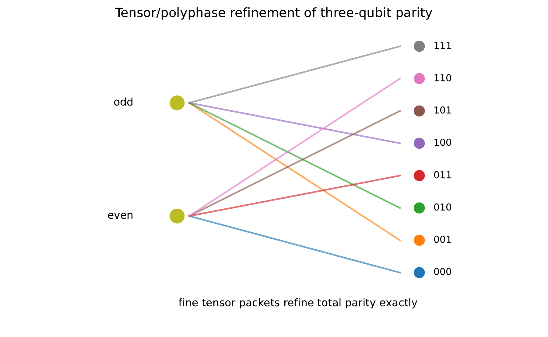
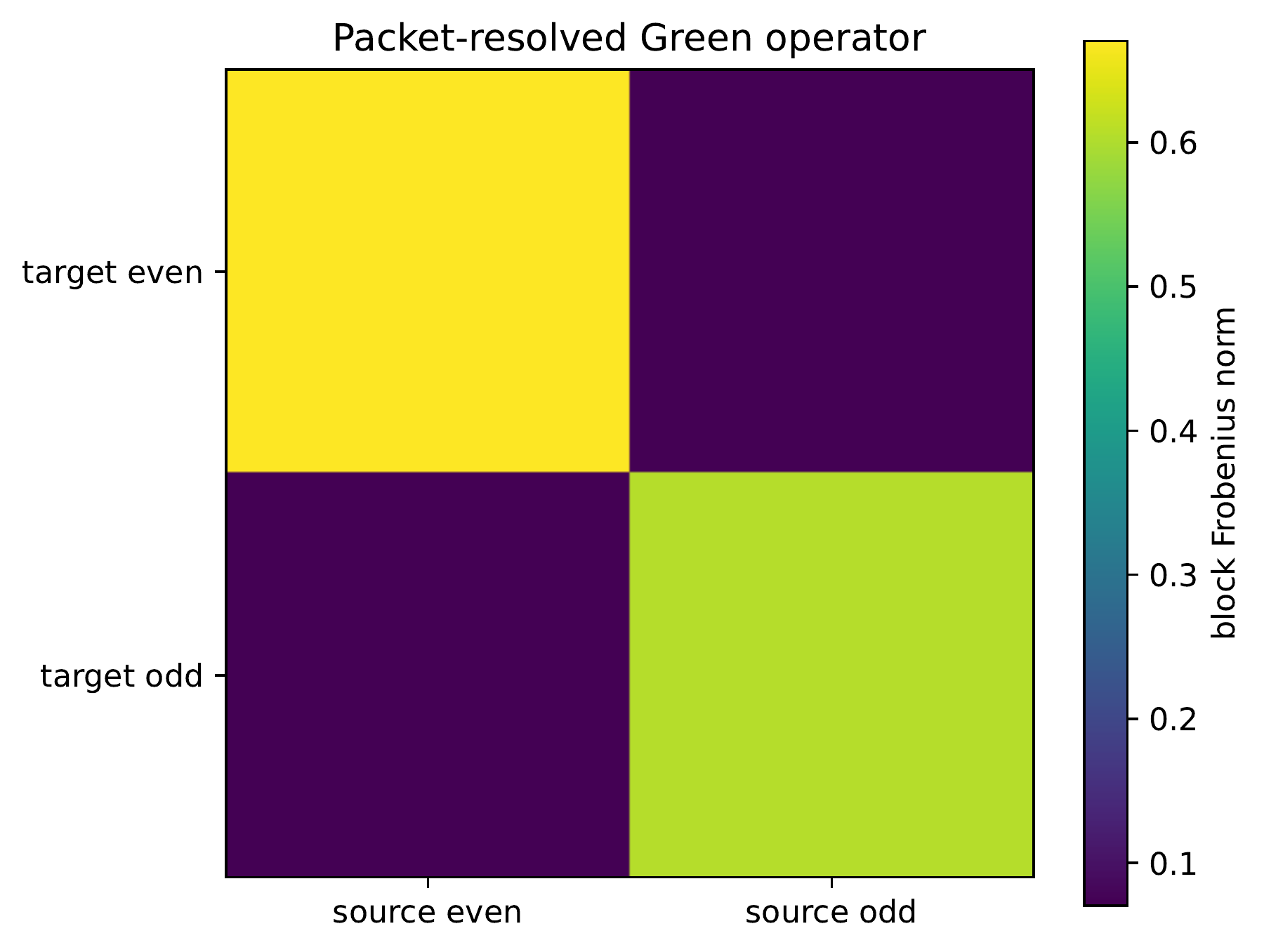
For parity,
\[
S=Z^{\otimes n},
\qquad
P_{\mathrm{even}}=\frac{I+S}{2},
\qquad
P_{\mathrm{odd}}=\frac{I-S}{2}.
\]
Permalink · Source line 227
I.3.2 Tensor refinement
On this page · Permalink · Source line 236
Fix \(N\ge1\). Suppose every factor \(a\) has a complete orthogonal family \(P^{(a)}_0,\ldots,P^{(a)}_{N-1}\). The fine tensor packets are
\[
P_{\mathbf j}^{\mathrm{fine}}
=
P^{(1)}_{j_1}\otimes\cdots\otimes P^{(m)}_{j_m}.
\]
Permalink · Source line 238
I.4 Quantum circuits as packet paths
On this page · Permalink · Source line 273
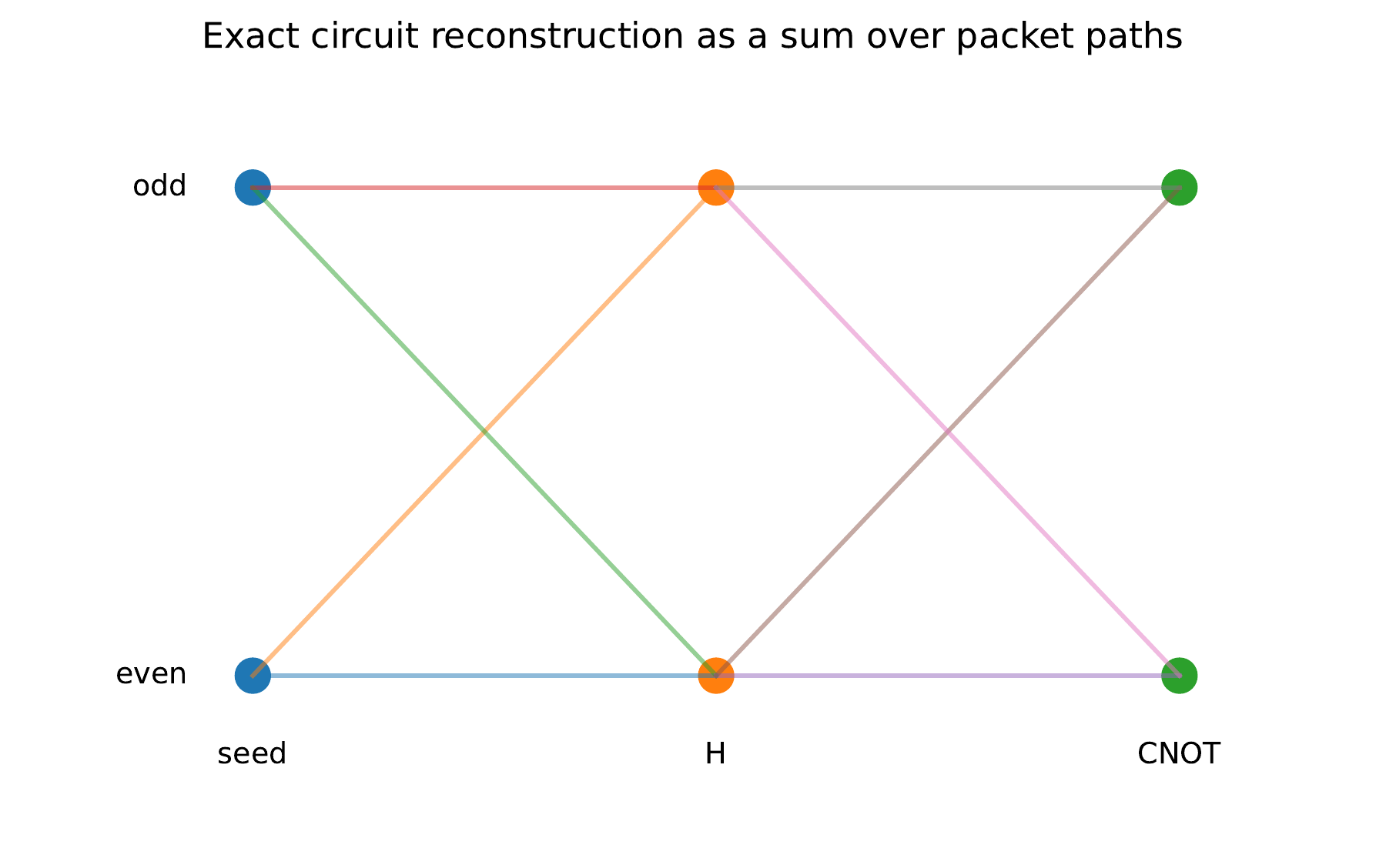
Let
\[
U=U_mU_{m-1}\cdots U_1
\]
be a circuit with \(m\ge1\), and let \(\{P_\alpha\}\) be a complete packet system. For the empty circuit \(m=0\), set \(U=I\). Its boundary block is \(P_\beta P_\alpha=\delta_{\beta\alpha}P_\alpha\).
Permalink · Source line 275
Example I.4.3: Bell seed circuit
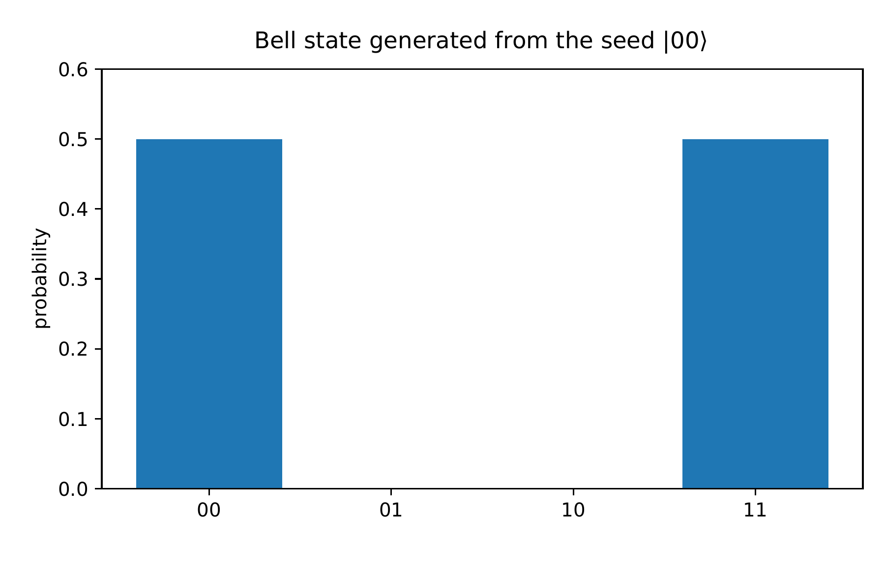
In this example only, \(H\) denotes the Hadamard gate, not a Hamiltonian. Starting from \({\left|00\right\rangle}\),
\[
(H\otimes I){\left|00\right\rangle}
=
\frac{{\left|00\right\rangle}+{\left|10\right\rangle}}{\sqrt2},
\]
and then
\[
\operatorname{CNOT}(H\otimes I){\left|00\right\rangle}
=
\frac{{\left|00\right\rangle}+{\left|11\right\rangle}}{\sqrt2}.
\]
The parity packets show that the final state lies entirely in the even sector, while the intermediate circuit path passes through both even and odd addresses.
Permalink · Source line 329
I.5 Symmetry-resolved Hamiltonians and leakage
On this page · Permalink · Source line 365
Let \(H=H^*\) and let \(P\) be a packet projector. If \([H,P]=0\), then \(P{\mathcal H}\) is invariant under \(e^{-itH}\).
Permalink · Source line 367
For two qubits and real parameters \(J,h\), consider
\[
H
=
JX\otimes X
+h(Z\otimes I+I\otimes Z).
\]
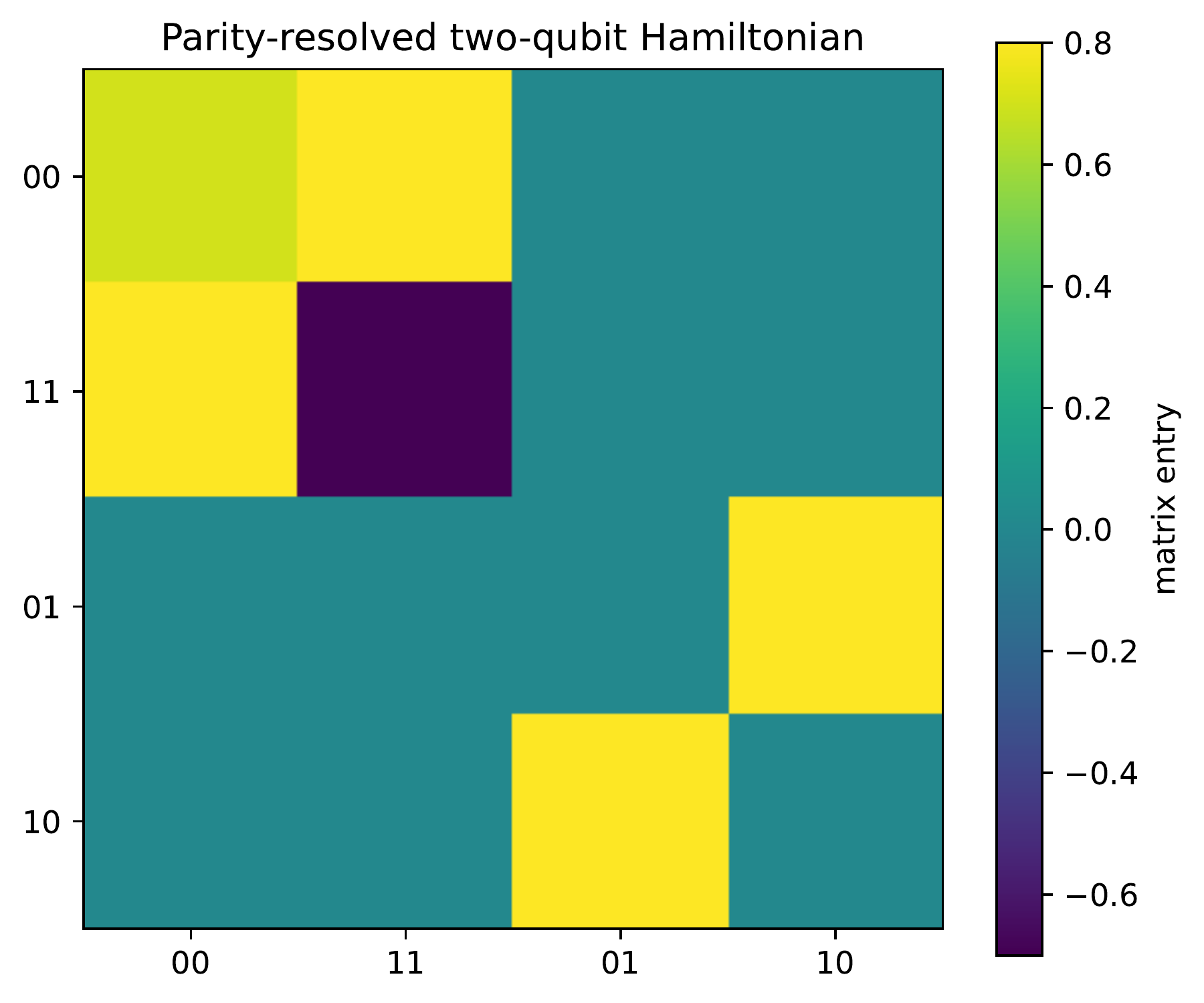
In the ordered even basis \(\{{\left|00\right\rangle},{\left|11\right\rangle}\}\) and odd basis \(\{{\left|01\right\rangle},{\left|10\right\rangle}\}\),
\[
H_{\mathrm{even}}
=
\begin{pmatrix}
2h&J\\
J&-2h
\end{pmatrix},
\qquad
H_{\mathrm{odd}}
=
\begin{pmatrix}
0&J\\
J&0
\end{pmatrix}.
\]
Therefore
\[
{\operatorname{Spec}} H_{\mathrm{even}}
=\{\pm\sqrt{4h^2+J^2}\},
\qquad
{\operatorname{Spec}} H_{\mathrm{odd}}=\{\pm J\}.
\]
Permalink · Source line 387
I.5.1 Leakage under broken symmetry
On this page · Permalink · Source line 425
Proof of Theorem I.5.2
Set \(F(s)=e^{isH}Pe^{-isH}\). Differentiating the exponential gives
\[
F'(s)=i\,e^{isH}[H,P]e^{-isH},\qquad F(0)=P.
\]
Unitary conjugation preserves the operator norm, so \(\|F'(s)\|=\|[H,P]\|\). The mean-value estimate on the interval between \(0\) and \(t\) yields
\[
\|F(t)-P\|\le |t|\,\|[H,P]\|.
\]
Finally, \(e^{itH}Qe^{-itH}P=(P-F(t))P\) and \(\|P\|\le1\). Left multiplication by \(e^{itH}\) preserves the norm and gives the desired inequality. This argument includes positive, negative, and zero time.
Back to statement · Read statement and proof side by side · Permalink · Source line 441 · Claim record · Lean coverage · Code · Worked examples
Numerical certificate I.5.3: Symmetry and negative control
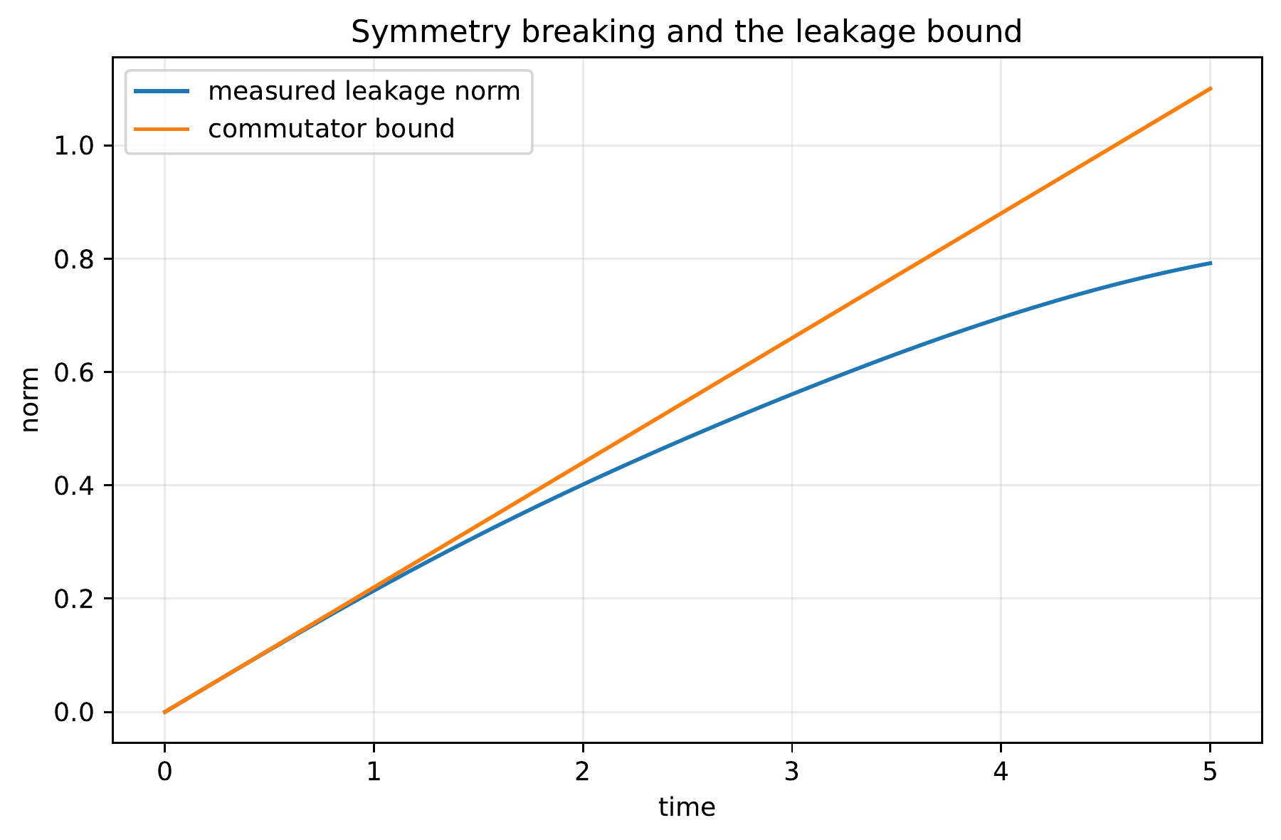
For the Hamiltonian that preserves parity, the norm of the block between distinct packets and the maximum measured leakage were both \(0\). Adding an \(X\otimes I\) perturbation broke parity and produced a maximum leakage of approximately \(0.79196\). The maximum violation of the proved bound remained \(0\).
Permalink · Source line 460 · Claim record · Lean coverage · Code · Worked examples
I.6 Moving packets, connections, and curvature
On this page · Permalink · Source line 464
I.6.1 Moving quantum coordinates
On this page · Permalink · Source line 466
I.6.2 A canonical projector connection
On this page · Permalink · Source line 507
Let \(P_1(t),\ldots,P_m(t)\) be differentiable on an open real time interval, with \(P_a(t)^*=P_a(t)\) and
\[
P_aP_b=\delta_{ab}P_a,
\qquad
\sum_aP_a=I.
\]
Permalink · Source line 509
Proof of Theorem I.6.3
Differentiating \(P_a^2=P_a\) gives
\[
\dot P_aP_a+P_a\dot P_a=\dot P_a.
\]
Summing over \(a\) and using \(\sum_a\dot P_a=0\) yields
\[
\sum_aP_a\dot P_a=-\sum_a\dot P_aP_a,
\]
which proves both displayed formulas for \(C\) and its skew-Hermiticity.
For fixed \(b\),
\[
CP_b=\dot P_bP_b.
\]
When \(a\ne b\), differentiating \(P_bP_a=0\) gives
\[
P_b\dot P_a=-\dot P_bP_a.
\]
Hence
\[
P_bC
=\sum_aP_b\dot P_aP_a
=-\dot P_b(I-P_b),
\]
and subtraction gives \([C,P_b]=\dot P_b\).
Back to statement · Read statement and proof side by side · Permalink · Source line 540 · Claim record · Lean coverage · Code · Worked examples
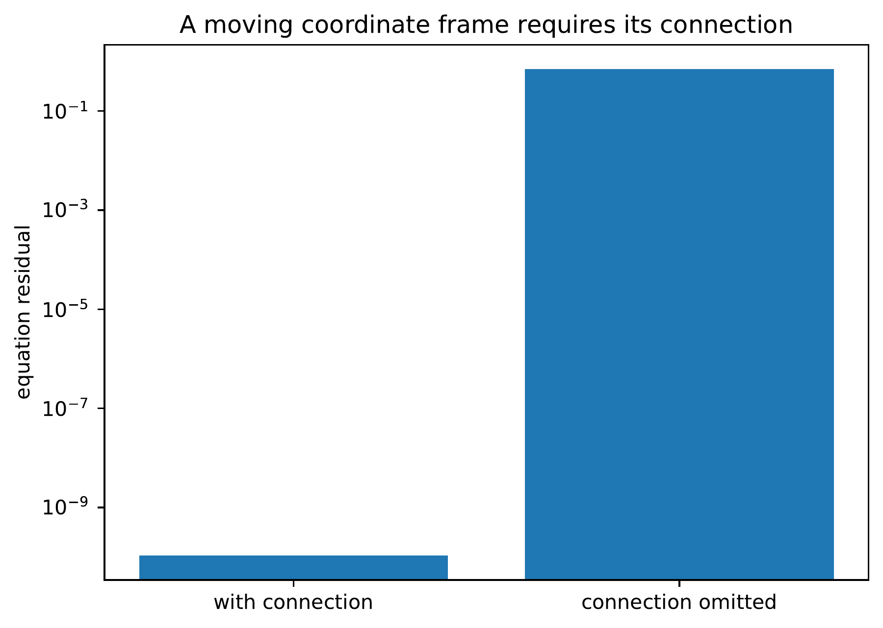
The connection generates infinitesimal transport of the moving packet frame. The packet family determines it directly, so its construction does not require a basis inside any packet.
Permalink · Source line 568
I.6.3 Projector curvature
On this page · Permalink · Source line 570
Classical input I.6.4: Projected connection
Let \(M\) be a smooth finite-dimensional real manifold without boundary, let \(V\) be a finite-dimensional real normed vector space, and let \(P:M\to\operatorname{End}_{{\mathbb R}}(V)\) be smooth with \(P(x)^2=P(x)\). In the quantum application, \(V\) is the underlying real space of a finite complex Hilbert space and \(P\) is an orthogonal complex-linear projector.
The rank of \(P\) is locally constant. On each open rank region, its ranges form a smooth vector bundle. For a smooth range section \(s\), so that \(Ps=s\), define
\[
\nabla_Xs=P\,ds(X).
\]
This is a connection on smooth range sections. For smooth vector fields \(X,Y\), its curvature satisfies
\[
\boxed{
(\nabla_X\nabla_Y-\nabla_Y\nabla_X-\nabla_{[X,Y]})s
=P[dP(X),dP(Y)]P\,s.
}
\]
Equivalently, its endomorphism-valued curvature is
\[
\boxed{F=P(dP\wedge dP)P.}
\]
No global frame or globally constant rank is required, and the vector fields need not commute. The geometric formalization concerns real smooth structures. It does not cover complex analytic manifolds or extensions to a boundary.
Read proof · Read statement and proof side by side · Permalink · Source line 572 · Claim record · Lean coverage · Code · Worked examples
Proof of Classical input I.6.4
Range coordinates. Fix \(a\in M\) and put
\[
T_a(x)=P(x)P(a)+(I-P(x))(I-P(a)).
\]
Then \(T_a(a)=I\) and \(P(x)T_a(x)=T_a(x)P(a)\). Invertibility is open, so on a neighborhood of \(a\), \(T_a(x)\) restricts to an isomorphism from \({\operatorname{Ran}} P(a)\) to \({\operatorname{Ran}} P(x)\). This proves local constancy of rank. The local coordinates and their transitions are
\[
(x,v)\longmapsto (x,T_a(x)^{-1}v),\qquad
u\longmapsto T_b(x)^{-1}T_a(x)u.
\]
Their smoothness follows from smoothness of \(P\) and inversion. The transition maps satisfy the cocycle identity by cancellation. These charts construct the smooth range bundles on the open rank regions, including when different connected components have different ranks.
Connection rules. Smoothness of \(P\,ds(X)\) and \(P^2=P\) show that \(\nabla_Xs\) is a smooth range section. Differentiation and projection give
\[
\begin{aligned}
\nabla_{X+Y}s&=\nabla_Xs+\nabla_Ys,&
\nabla_{fX}s&=f\nabla_Xs,\\
\nabla_X(s+t)&=\nabla_Xs+\nabla_Xt,&
\nabla_X(fs)&=f\nabla_Xs+(Xf)s
\end{aligned}
\]
for smooth real \(f\). The range coordinates above identify ambient smooth range sections with smooth sections of the constructed bundle.
Curvature. Differentiating \(P^2=P\) gives \(P(dP(X))P=0\). Write \(D_Xs=ds(X)\). For ambient smooth sections,
\[
D_XD_Ys-D_YD_Xs-D_{[X,Y]}s=0.
\]
Expansion of the projected derivatives therefore leaves
\[
R(X,Y)s=P(dP(X))D_Ys-P(dP(Y))D_Xs.
\]
Since \(Ps=s\), differentiation gives \(D_Ys=(dP(Y))s+PD_Ys\). The terms with a middle \(P\) vanish. Thus
\[
R(X,Y)s=P\bigl(dP(X)dP(Y)-dP(Y)dP(X)\bigr)P\,s.
\]
This expression is alternating and bilinear in the tangent vectors, and it preserves the range. The ordinary chain rule and the transformation law for the Lie bracket make the local calculations agree on chart overlaps, which gives the global formula.
Back to statement · Read statement and proof side by side · Permalink · Source line 593 · Claim record · Lean coverage · Code · Worked examples
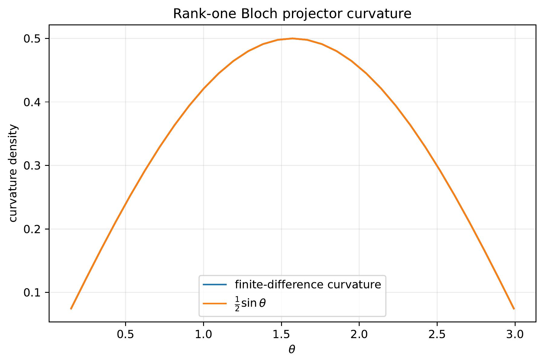
For an orthogonal rank-one complex projector, use the scalar connection convention \(A=-i\langle u,du\rangle\) in a local unit frame. The associated scalar curvature density is
\[
{\mathcal F}_{\mu\nu}
=-i{\operatorname{Tr}}\left(P[\partial_\mu P,\partial_\nu P]\right).
\]
On the Bloch sphere,
\[
P(\theta,\phi)
=
\frac12\left(I+\mathbf n(\theta,\phi)\cdot\boldsymbol\sigma\right),
\]
where
\[
\mathbf n=(\sin\theta\cos\phi,\sin\theta\sin\phi,\cos\theta).
\]
The Pauli multiplication law gives
\[
[\partial_\theta P,\partial_\phi P]
=\frac{i}{2}(\partial_\theta\mathbf n\mathbin{\times}\partial_\phi\mathbf n)\cdot\boldsymbol\sigma.
\]
Using \({\operatorname{Tr}}(P\,\mathbf a\cdot\boldsymbol\sigma)=\mathbf n\cdot\mathbf a\) therefore yields
\[
\boxed{{\mathcal F}_{\theta\phi}
=\frac12\mathbf n\cdot(\partial_\theta\mathbf n\mathbin{\times}\partial_\phi\mathbf n)
=\frac12\sin\theta.}
\]
The scalar sign changes if the opposite convention for \(A\) is chosen. This explicit calculation is not a separate entry among the 19 items in the Lean register.
Permalink · Source line 631
I.7 Measurements and quantum channels
On this page · Permalink · Source line 670
I.7.1 Packet measurements
On this page · Permalink · Source line 672
Let \(\rho\) be a density matrix and let \(\{E_k\}\) be a POVM:
\[
E_k\ge0,
\qquad
\sum_kE_k=I.
\]
The outcome probabilities are
\[
p_k={\operatorname{Tr}}(E_k\rho).
\]
Permalink · Source line 674
The theorem identifies which coherences a declared measurement can detect. Observables that are diagonal in the packet decomposition cannot detect coherence between distinct packets. Coherence within a packet remains available to such observables.
Permalink · Source line 716
I.7.2 Kraus transfer
On this page · Permalink · Source line 718
A quantum channel can transfer both populations and coherences between packet addresses. A Kraus representation describes this transfer by summing the contributions of its individual branches. The normalization of those branches ensures that the total trace is preserved.
Permalink · Source line 720
Packet superoperator blocks are defined by
\[
\Phi_{\alpha\beta;\gamma\delta}(X)
=
P_\alpha
\Phi(P_\gamma XP_\delta)
P_\beta.
\]
Summing all four packet indices reconstructs \(\Phi(X)\) exactly.
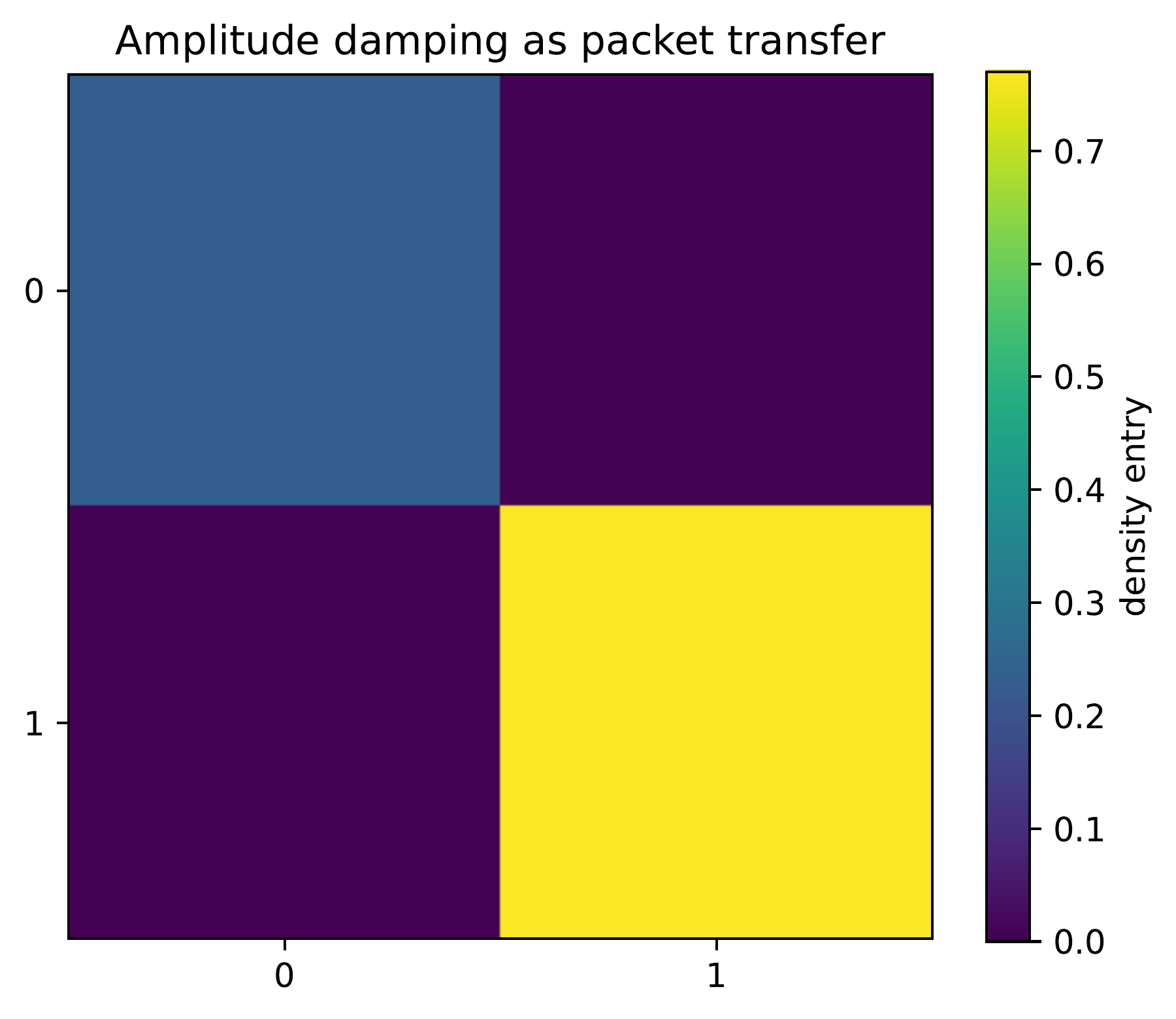
For amplitude damping with a real parameter \(0\le\gamma\le1\),
\[
K_0=
\begin{pmatrix}
1&0\\0&\sqrt{1-\gamma}
\end{pmatrix},
\qquad
K_1=
\begin{pmatrix}
0&\sqrt\gamma\\0&0
\end{pmatrix}.
\]
The excited state becomes
\[
\Phi({\left|1\right\rangle}{\left\langle1\right|})
=
\gamma{\left|0\right\rangle}{\left\langle0\right|}+(1-\gamma){\left|1\right\rangle}{\left\langle1\right|}.
\]
Permalink · Source line 750
Numerical certificate I.7.3: Channel reconstruction
For \(\gamma=0.23\), the residuals for Kraus completeness and the output trace were \(0\). The computed output from \({\left|1\right\rangle}{\left\langle1\right|}\) was \({\operatorname{diag}}(0.23,0.77)\). In the Bell state test, packet dephasing left every measurement probability in the computational basis unchanged.
Permalink · Source line 786 · Claim record · Lean coverage · Code · Worked examples
I.8 Quantum error correction as obstruction-packet annihilation
On this page · Permalink · Source line 790
Let \(P=P^*=P^2\) project onto a code space \({\mathcal C}\subset{\mathcal H}\), and let \(E_1,\ldots,E_r\) be a finite family of complex error matrices. Neither a nonzero code nor channel normalization is assumed unless stated. The operators
\[
P E_a^*E_bP
\]
are the obstruction packets on the code. If they retain information about the logical state beyond one scalar multiple of \(P\), the environment can distinguish logical states and exact correction is impossible.
We call a recovery complete when it is a Kraus map
\[
{\mathcal R}(X)=\sum_jK_jXK_j^*,\qquad \sum_jK_j^*K_j=I.
\]
The family is exactly correctable when one such recovery works for every coherent error combination \(A_w=\sum_aw_aE_a\): for every \(w\) there is a real \(t_w\ge0\), independent of the logical input, such that
\[
PXP=X\quad\Longrightarrow\quad
{\mathcal R}(A_wXA_w^*)=t_wX.
\]
The coefficient is an unnormalized weight. It is not necessarily a probability for an arbitrary matrix \(A_w\).
Permalink · Source line 792
Classical input I.8.1: Finite Knill–Laflamme criterion
The finite error family is exactly correctable in the sense just defined if and only if there is a positive semidefinite complex matrix \(C=(c_{ab})\) such that
\[
\boxed{PE_a^*E_bP=c_{ab}P\qquad\text{for every }a,b.}
\]
If \(\sum_aE_a^*E_a=I\), the equivalent normalized-channel formulation is the existence of a complete recovery satisfying
\[
{\mathcal R}\!\left(\sum_aE_aXE_a^*\right)=X
\quad\text{for every }X\text{ with }PXP=X.
\]
The zero code and an empty error family are included. An empty family cannot define a channel that preserves trace on a nonzero ambient space.
Read proof · Read statement and proof side by side · Permalink · Source line 809 · Claim record · Lean coverage · Code · Worked examples
Proof of Classical input I.8.1
Necessity. Fix an error \(E_a\) and let \(L_j=K_jE_aP\). Perfect recovery on rank-one code operators gives
\[
\sum_j{\left|L_j\psi\right\rangle}{\left\langle L_j\psi\right|}
=t_a{\left|\psi\right\rangle}{\left\langle\psi\right|}\qquad(\psi\in{\mathcal C}).
\]
For every vector orthogonal to \(\psi\), the quadratic form on the left is a sum of nonnegative squared absolute values and equals zero. Each \(L_j\psi\) therefore lies in the span of \(\psi\). A linear operator that preserves every line in \({\mathcal C}\) is scalar there: apply it to two independent vectors and their sum. The one-dimensional case is immediate, and the claim is vacuous for the zero code. Consequently
\[
K_jE_aP=d_{ja}P.
\]
Recovery completeness now gives
\[
\begin{aligned}
PE_a^*E_bP
&=\sum_j (K_jE_aP)^*(K_jE_bP)\\
&=\left(\sum_j\overline{d_{ja}}d_{jb}\right)P.
\end{aligned}
\]
The coefficients form a Gram matrix, hence are positive semidefinite. For a normalized channel, apply the same rank-one argument to all composite branches \(K_jE_aP\) at once to obtain the necessary condition.
Sufficiency. Diagonalize \(C=U\operatorname{diag}(\lambda_r)U^*\) with \(U\) unitary and \(\lambda_r\ge0\). Define compressed transformed errors
\[
F_r=\sum_aU_{ar}E_aP.
\]
Then \(F_rP=F_r\) and \(F_r^*F_s=\lambda_r\delta_{rs}P\). If \(\lambda_r=0\), \(F_r^*F_r=0\) forces \(F_r=0\). For positive eigenvalues only, set \(V_r=F_r/\sqrt{\lambda_r}\). These satisfy
\[
V_rP=V_r,\qquad V_r^*V_s=\delta_{rs}P.
\]
Let \(S=\sum_{\lambda_r>0}V_rV_r^*\). Orthogonality makes \(S\) an orthogonal projector. Use the recovery branches
\[
K_r=V_r^*,\qquad K_{\mathrm{unused}}=I-S.
\]
They are complete on the whole ambient space because
\[
\sum_rK_r^*K_r+K_{\mathrm{unused}}^*K_{\mathrm{unused}}
=S+(I-S)^2=I.
\]
The inverse unitary change of coordinates reconstructs each \(E_aP\) from the \(F_r\). Every recovery branch of a coherent combination is therefore scalar on the code, while the branch for the unused space vanishes. For all supported matrices, the resulting recovery is
\[
{\mathcal R}(A_wXA_w^*)=(w^*Cw)X.
\]
This establishes the arbitrary-family statement without assuming normalization. Under \(\sum_aE_a^*E_a=I\) and \(P\ne0\), summing the diagonal KL equations gives \({\operatorname{Tr}} C=1\), so the normalized-channel output is \(X\). When \(P=0\), every supported \(X\) is zero and the conclusion is automatic. The recovery is trace preserving by completeness and completely positive at every finite ancillary dimension by the Kraus calculation in Classical Input Classical input I.7.2.
Back to statement · Read statement and proof side by side · Permalink · Source line 822 · Claim record · Lean coverage · Code · Worked examples
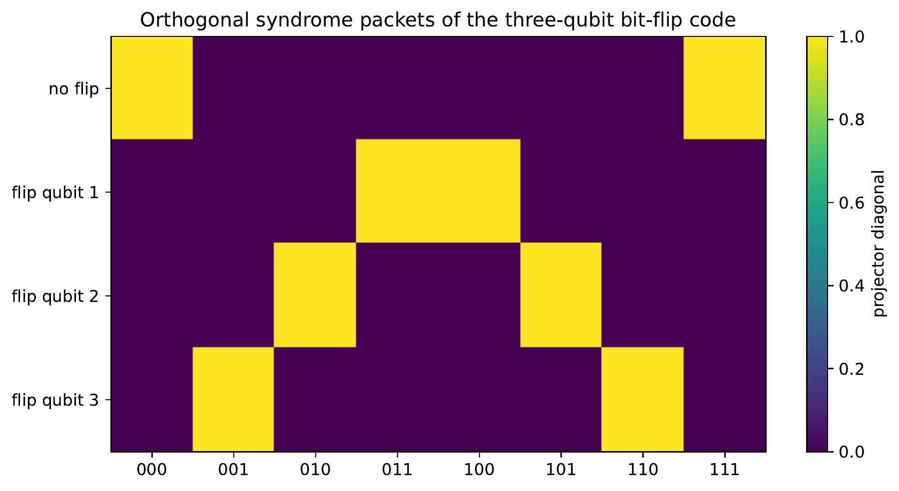
For the three-qubit bit-flip code,
\[
{\left|0_L\right\rangle}={\left|000\right\rangle},
\qquad
{\left|1_L\right\rangle}={\left|111\right\rangle},
\]
and the error family is
\[
I,
\quad X\otimes I\otimes I,
\quad I\otimes X\otimes I,
\quad I\otimes I\otimes X.
\]
The four error images of the code are pairwise orthogonal two-dimensional syndrome packets whose projectors sum to the identity on the eight-dimensional Hilbert space.
Permalink · Source line 866
Numerical certificate I.8.2: Exact bit-flip correction
The residuals for the Knill–Laflamme condition and completeness of the syndrome packets were both \(0\). A mixed channel of single bit flip errors, applied to a nontrivial logical superposition, was reversed with a residual of \(1.0385\times10^{-16}\) in the density matrix.
Permalink · Source line 888 · Claim record · Lean coverage · Code · Worked examples
I.9 Exact effective dynamics
On this page · Permalink · Source line 892
I.9.1 Schur–Feshbach reduction
On this page · Permalink · Source line 894
Let \(P\) be a retained packet projector and \(Q=I-P\). In packet coordinates,
\[
H=
\begin{pmatrix}
H_{PP}&H_{PQ}\\
H_{QP}&H_{QQ}
\end{pmatrix}.
\]
Permalink · Source line 896
Theorem I.9.1: Exact Feshbach resolvent
Assume that both \(zI_Q-H_{QQ}\) and \(zI-H\) are invertible. Define
\[
\boxed{
H_{\mathrm{eff}}(z)
=
H_{PP}
+H_{PQ}(z-H_{QQ})^{-1}H_{QP}.
}
\]
Then
\[
\boxed{
P(z-H)^{-1}P
=
\left(z-H_{\mathrm{eff}}(z)\right)^{-1}
}
\]
where the left side is restricted to \(P{\mathcal H}\), the right side is an inverse on that retained space, and both are written in the same orthonormal basis. Here \(z-H_{QQ}\) and \(z-H_{\mathrm{eff}}\) abbreviate the appropriately sized scalar matrices minus the indicated blocks.
Read proof · Read statement and proof side by side · Permalink · Source line 905 · Claim record · Lean coverage · Code · Worked examples
The second premise cannot be dropped: at \(z=0\) and \(H=\operatorname{diag}(0,-1)\), the eliminated block is \(1\) but \(zI-H\) is singular. This counterexample is also included in the Lean module.
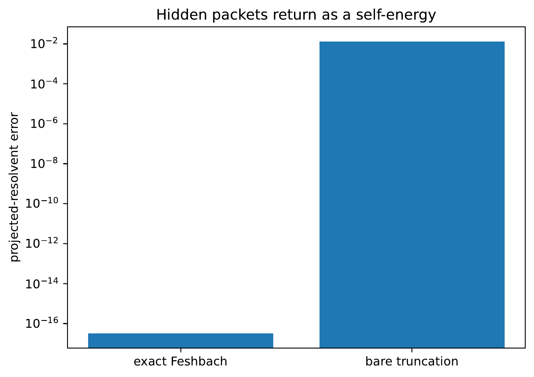
The self-energy
\[
\Sigma_P(z)
=H_{PQ}(z-H_{QQ})^{-1}H_{QP}
\]
contains the complete influence of the eliminated packet. Bare truncation drops \(\Sigma_P(z)\) and is therefore exact only when the coupling between packets vanishes or the self-energy cancels for another stated reason.
Permalink · Source line 934
I.9.2 The hidden packet as memory
On this page · Permalink · Source line 963
For a time-independent finite Hamiltonian \(H\) and fixed projectors \(P,Q\), write \(\psi=x+y\), with \(x=P\psi\) and \(y=Q\psi\). Then
\[
\begin{aligned}
i\dot x&=H_{PP}x+H_{PQ}y,\\
i\dot y&=H_{QP}x+H_{QQ}y.
\end{aligned}
\]
Solving the second equation gives
\[
y(t)
=e^{-itH_{QQ}}y(0)
-i\int_0^t e^{-i(t-s)H_{QQ}}H_{QP}x(s)\,ds.
\]
Substitution yields the exact Volterra equation
\[
\boxed{
\begin{aligned}
i\dot x(t)
={}&H_{PP}x(t)
+H_{PQ}e^{-itH_{QQ}}y(0)\\
&-i\int_0^t
K(t-s)x(s)\,ds,
\end{aligned}
}
\]
with memory kernel
\[
\boxed{
K(t)=H_{PQ}e^{-itH_{QQ}}H_{QP}.
}
\]
The influence of the eliminated degrees of freedom is therefore retained in a self-energy that depends on frequency, or equivalently in an exact memory term. For forward evolution the integral is causal. When the Hamiltonian depends on time, the corresponding propagator between two times replaces the stationary exponential used here. This Volterra derivation is not a separate entry in the finite Lean register.
Permalink · Source line 965
I.10 Finite quantum geometry
On this page · Permalink · Source line 998
I.10.1 A projector-resolved geometry
On this page · Permalink · Source line 1000
At resolution \(\ell\), define
\[
\boxed{
\mathfrak Q_\ell
=
\left(
{\mathcal A}_\ell,
{\mathcal H}_\ell,
D_\ell,
\{P_{\ell,\alpha}\},
E_\ell,
C_\ell,
\Pi_\ell^{\mathrm{phys}},
T_\ell
\right).
}
\]
In order, the entries specify the observable algebra, Hilbert space, geometric or Dirac-type operator, packet projectors, embedding into the fine space, reconstruction onto the coarse space, physical constraint projector, and transfer operator. The maps have types \(E_\ell:{\mathcal H}_\ell\to{\mathcal H}_{\ell+1}\) and \(C_\ell:{\mathcal H}_{\ell+1}\to{\mathcal H}_\ell\). The left inverse relation \(C_\ell E_\ell=I\) alone does not imply \(C_\ell=E_\ell^*\) or make the embedding isometric.
A coherent refinement should satisfy
\[
C_\ell E_\ell=I
\]
and
\[
\boxed{
P_{\ell,\alpha}
=
C_\ell
\left(
\sum_{\beta\succ\alpha}P_{\ell+1,\beta}
\right)
E_\ell.
}
\]
For an operator \(D\), define the refinement defect
\[
\Delta_\ell(D)
=C_\ell D_{\ell+1}E_\ell-D_\ell.
\]
Exact resolution independence is \(\Delta_\ell(D)=0\). When exact equality is too strong, the correct continuum problem is to prove convergence of the resolvents and uniform control of the effective self-energies.
Permalink · Source line 1002
I.10.2 Euclidean transfer
On this page · Permalink · Source line 1052
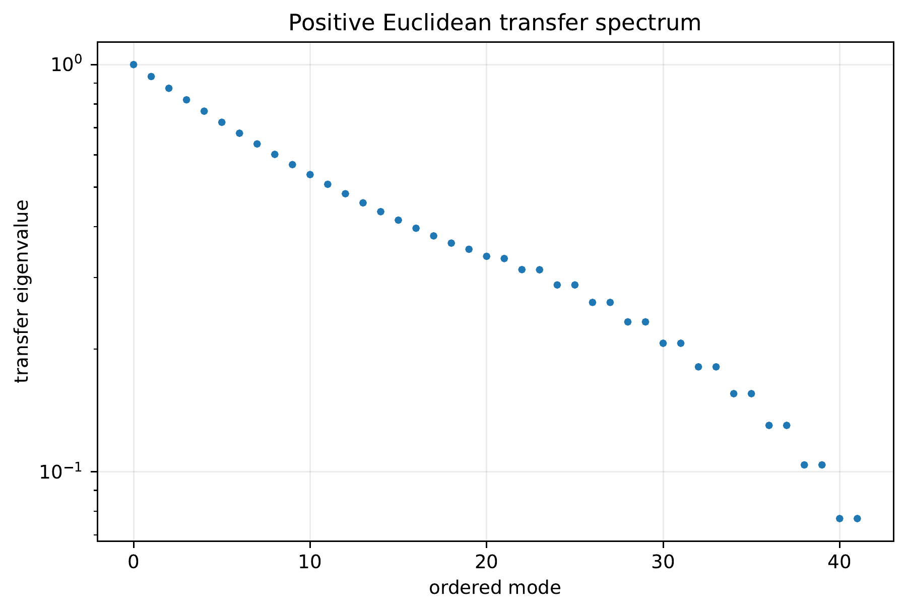
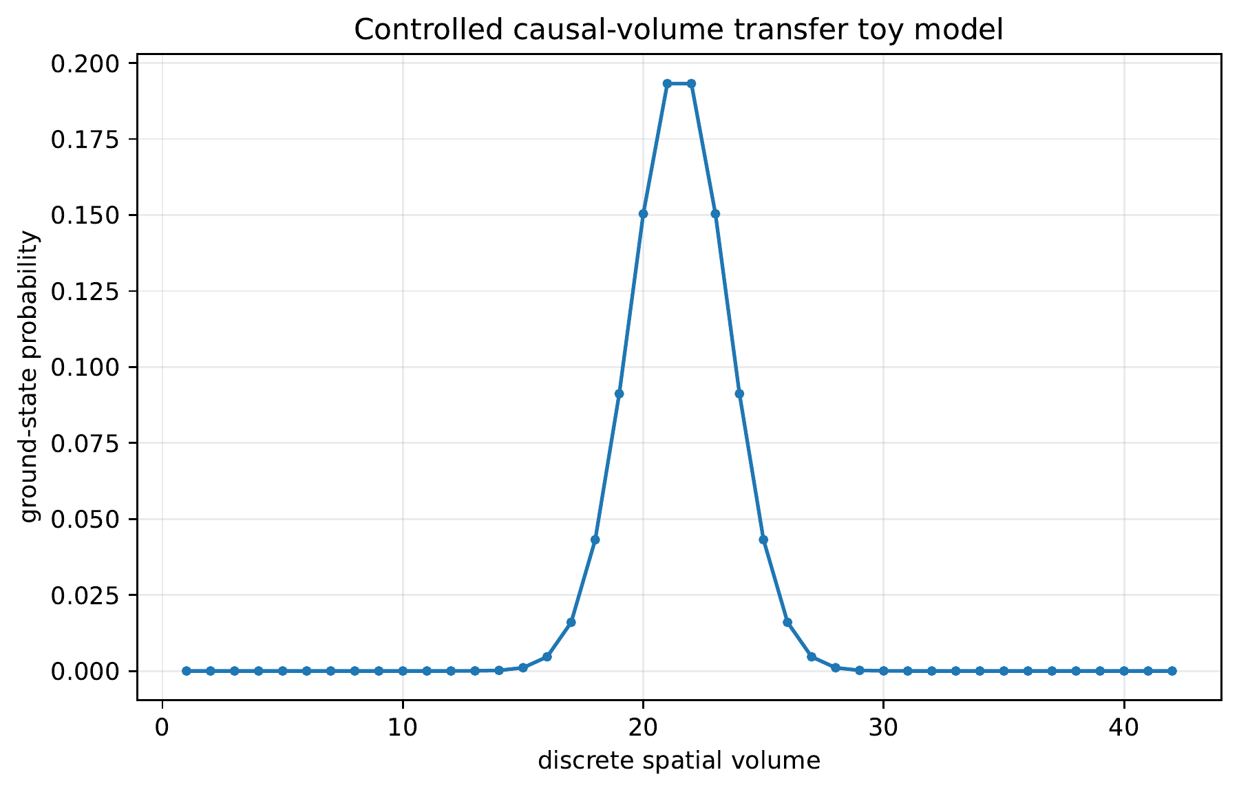
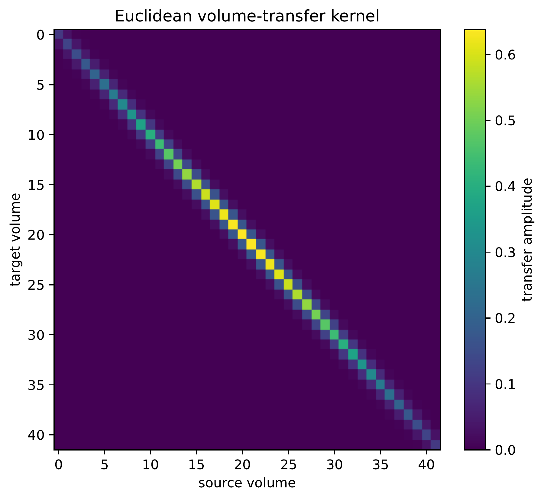
The paper tests a controlled volume-state model
\[
H_{nn}=2\kappa+V(n),
\qquad
H_{n,n+1}=H_{n+1,n}=-\kappa,
\]
with \(\kappa>0\) and a real confining potential. This is a finite transfer-matrix test only. Operator positivity alone is not reflection positivity of a Euclidean field measure. It is not derived from a gravitational path integral and is not evidence for a unique microscopic spacetime dynamics.
Permalink · Source line 1078
I.11 Spectral dimension and continuum diagnostics
On this page · Permalink · Source line 1113
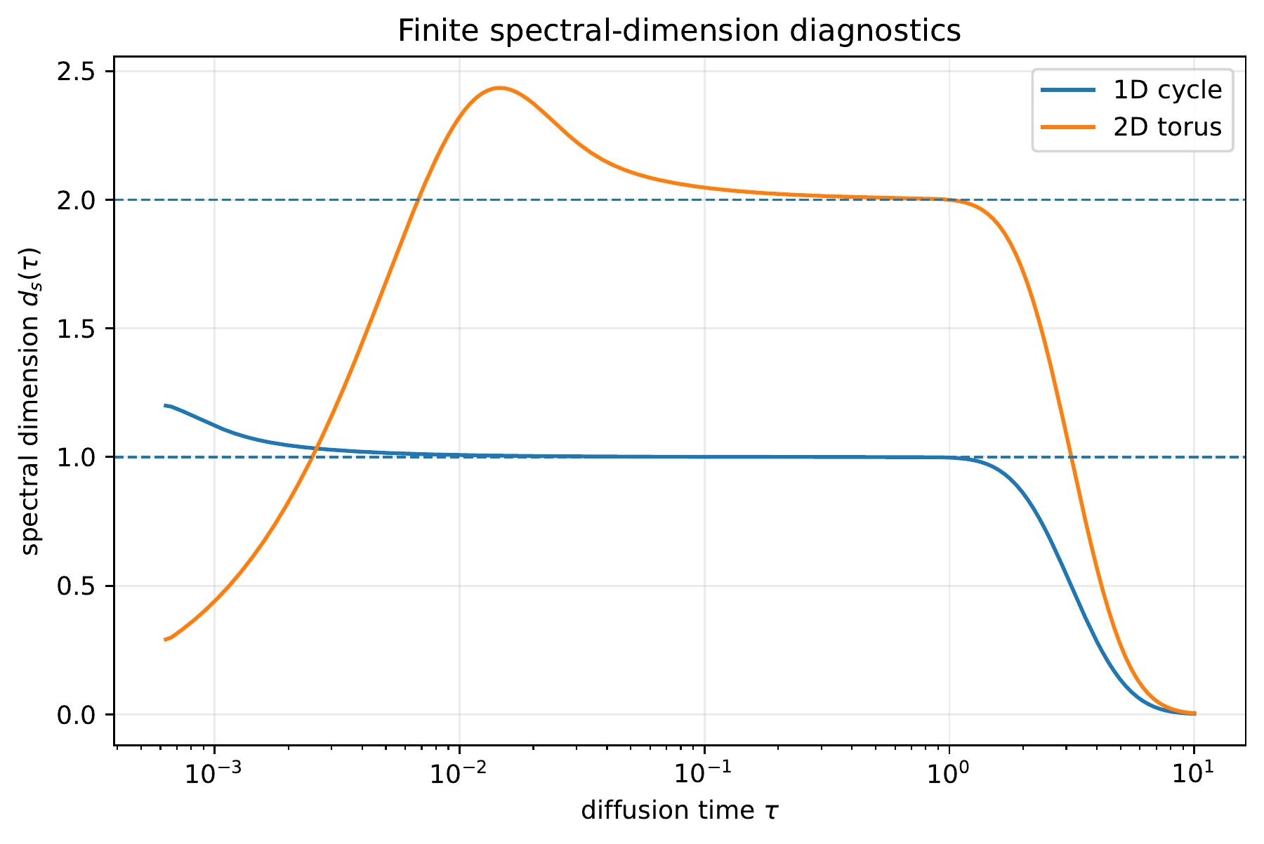
Let \(L\ge0\) be a finite Laplacian on \(N\ge1\) states, with eigenvalues \(\lambda_j\) and at least one zero eigenvalue. For diffusion time \(\tau>0\), define the normalized heat trace
\[
K(\tau)=\frac1N\sum_j e^{-\tau\lambda_j}
\]
and the scale-dependent spectral dimension
\[
\boxed{
d_s(\tau)
=-2\frac{d\log K(\tau)}{d\log\tau}.
}
\]
For a finite system, \(d_s(\tau)\) is a diagnostic, not a topological invariant. Indeed, finite differentiation gives
\[
d_s(\tau)=2\tau\,
\frac{\sum_j\lambda_j e^{-\tau\lambda_j}}{\sum_j e^{-\tau\lambda_j}}.
\]
It tends to zero as \(\tau\downarrow0\) and, under the stated assumption of a zero mode, as \(\tau\to\infty\). If a general positive operator has no zero mode, its behavior at large times is instead asymptotic to \(2\tau\lambda_{\min}\). The conclusion for operators with a zero mode therefore does not apply to that case. Inferring a geometric dimension requires a stable intermediate window and a controlled refinement limit.
Permalink · Source line 1115
I.11.1 The circle dispersion bound
On this page · Permalink · Source line 1133
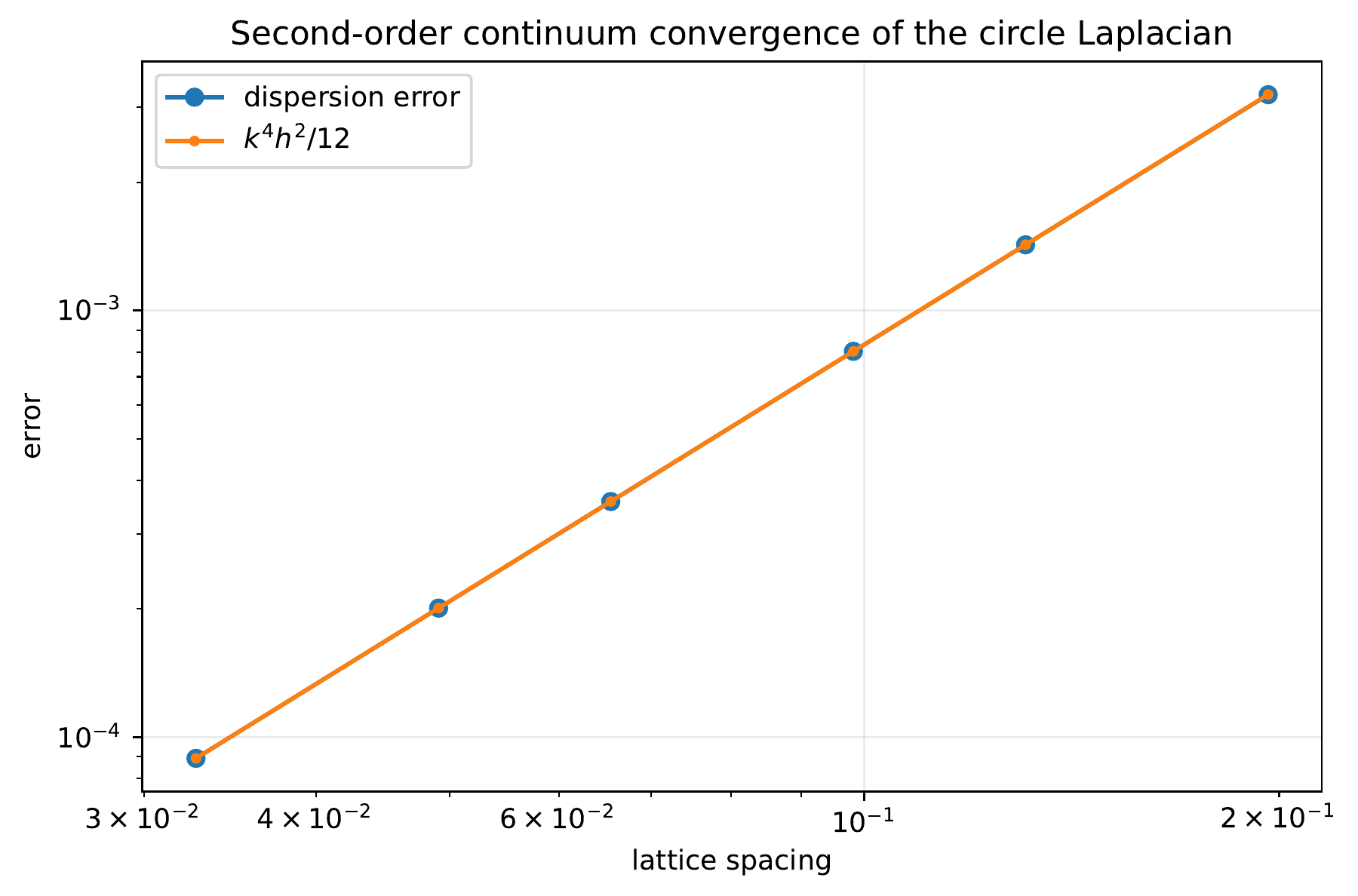
For a periodic grid with spacing \(h>0\) and physical wave number \(k\in{\mathbb R}\),
\[
\lambda_{k,h}
=
\frac4{h^2}\sin^2\left(\frac{kh}{2}\right).
\]
Permalink · Source line 1135
Proof of Theorem I.11.1
Put \(x=kh/2\). The inequalities \(|\sin x|\le|x|\) and \(|x-\sin x|\le |x|^3/6\), which hold for every real argument, give
\[
0\le x^2-\sin^2x
=|x-\sin x|\,|x+\sin x|
\le\frac{|x|^3}{6}\,2|x|
=\frac{x^4}{3}.
\]
Multiplying by \(4/h^2\) proves both bounds. The estimate holds for every frequency. Its interpretation as convergence of second order keeps \(k\) fixed while \(h\to0\), so it does not assert a uniformly small relative error across all grid modes.
Back to statement · Read statement and proof side by side · Permalink · Source line 1153 · Claim record · Lean coverage · Code · Worked examples
I.11.2 One- and two-dimensional plateaus
On this page · Permalink · Source line 1175
At intermediate diffusion times, a finite cycle and a finite torus can exhibit plateaus near the dimensions of their underlying geometries. The following figure and numerical certificate show the reported behavior for these two examples. The plateaus occur between the small and large time regimes in which the spectral dimension returns to zero.
Permalink · Source line 1177
Numerical certificate I.11.3: Spectral dimension
The median intermediate plateaus were
\[
d_s^{(1)}=1.00062,
\qquad
d_s^{(2)}=2.03781.
\]
These tests recover the expected dimensions of the chosen finite geometries. They do not select a physical theory of quantum spacetime.
Permalink · Source line 1186 · Claim record · Lean coverage · Code · Worked examples
I.12 Constraint packets and the quantum-spacetime boundary
On this page · Permalink · Source line 1196
At one finite level, let \(\widehat C_A\) be a finite family of matrix constraints, with fixed scalar structure coefficients, and let \(\Pi^{\mathrm{phys}}\) be the orthogonal projector onto their exact common kernel. If the classical constraint algebra has structure coefficients \(f_{AB}^{\ \ C}\), define the anomaly operator
\[
\boxed{
\mathfrak A_{AB}
=
[\widehat C_A,\widehat C_B]
-i\sum_C f_{AB}^{\ \ C}\widehat C_C.
}
\]
Its physical packet is
\[
\Pi^{\mathrm{phys}}\mathfrak A_{AB}\Pi^{\mathrm{phys}}.
\]
In this exact finite setting, \(\widehat C_C\Pi^{\mathrm{phys}}=0\) for every \(C\). Associativity gives
\[
\mathfrak A_{AB}\Pi^{\mathrm{phys}}=0,
\qquad
\Pi^{\mathrm{phys}}\mathfrak A_{AB}\Pi^{\mathrm{phys}}=0
\]
automatically. This compression therefore cannot certify operator closure away from the physical range. A nonzero measured compression contradicts the exact-kernel assumptions or indicates an approximation or implementation error. For example, \(C_1=\operatorname{diag}(1,0,0)\) and \(C_2=E_{12}+E_{21}\) annihilate the same third coordinate, while their commutator \(E_{12}-E_{21}\) is nonzero. With zero proposed structure coefficients, the anomaly is nonzero but its physical compression vanishes.
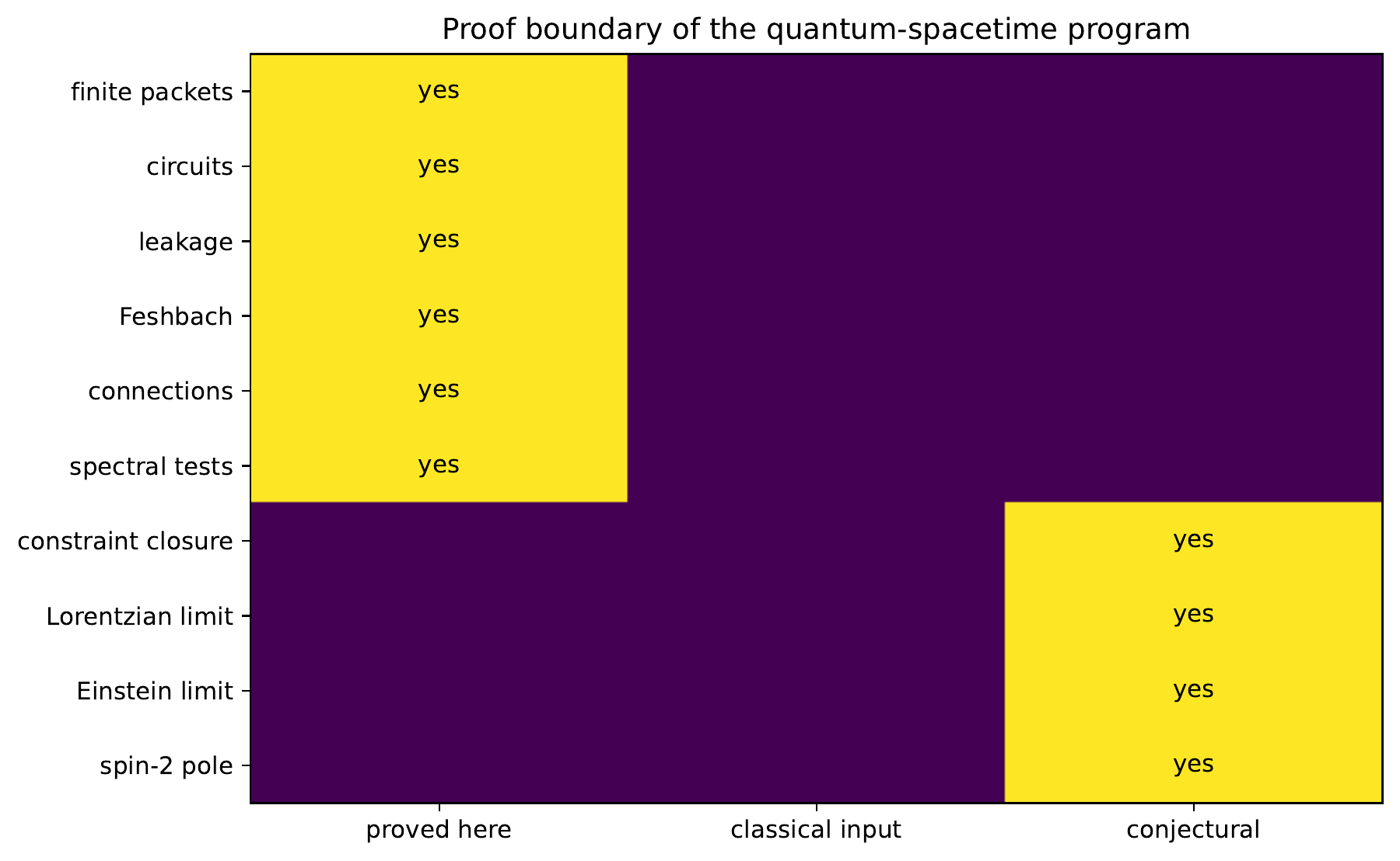
The closure target must be stated at the operator level, not inferred from that automatic compression. Unbounded constraints additionally require a specified common invariant domain. Neither such a domain theory nor gravitational structure functions are supplied by the finite check.
Permalink · Source line 1198
Conjecture I.12.1: Anomaly-free refinement
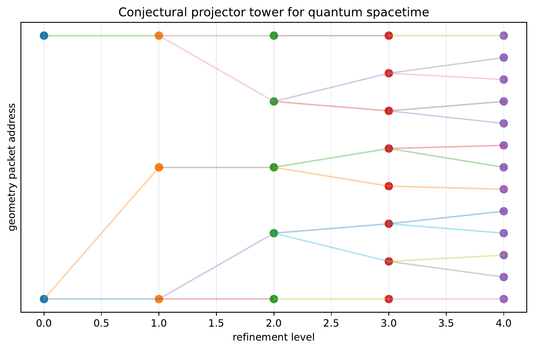
For a specified nontrivial quantum-geometric constraint model, there exists a coherent packet tower with nonzero physical spaces, compatible physical projectors, and exact operator closure
\[
\mathfrak A^{(\ell)}_{AB}=0
\]
at every finite level. The compatible physical compression then vanishes as a consequence, not as a substitute for closure.
Permalink · Source line 1221 · Claim record · Lean coverage · Code · Worked examples
The substantive research target is the operator condition. The earlier condition stated only in terms of compression was too weak. A choice of model, dynamics, and refinement maps is still needed before this program becomes a fully specified physical existence problem.
Permalink · Source line 1228
Conjecture I.12.2: Uniform Feshbach control
For the same specified tower, the self-energies from exact elimination of fine packets admit bounds uniform in cutoff and volume on a common spectral domain. Together with consistent identifications of the Hilbert spaces and a proved resolvent convergence criterion, they yield a nontrivial continuum limit in the strong resolvent sense. Uniform boundedness alone is not asserted to imply convergence.
Permalink · Source line 1230 · Claim record · Lean coverage · Code · Worked examples
The exact finite identities establish none of these physical conclusions, and no formal theorem of logical independence is claimed. Exact packet reconstruction provides a kinematic and computational advantage. It does not determine the physical action, prove existence of the continuum theory, or guarantee the limit of general relativity.
Permalink · Source line 1251