Large Signal ModelReading edition

18. A complete output-only identification example

Reading tools
Reading libraryFind statementsInspect Lean
Switch work

Saved reading

Read side by side

Start reading

Resources & source

Original TeX with line links · Download TeX

The wording and mathematics follow the retained manuscript. This reading format does not add a proof review or extend Lean coverage.

Skip contents and start reading

18. A complete output-only identification example

Return to the rational system from Section 13, now with an additional independent hidden coordinate:

\[ L=\begin{pmatrix} 1/2&1&0\\ 1/4&1/3&0\\ 0&0&5/6 \end{pmatrix}, \qquad C=\begin{pmatrix}1&0&0\end{pmatrix}. \]

The third coordinate never influences the observed output. The first coordinate alone is not closed, but

\[ O_2=\begin{pmatrix}1&0&0\\1/2&1&0\end{pmatrix} \]

has rank two and \(O_3\) has the same rank. Proposition 14 gives an exact two-dimensional delay state. Choose \(x_0=(1,0,q)^\top\) for any \(q\). The first four observations are

\[ y_0=1,\quad y_1=1/2,\quad y_2=1/2,\quad y_3=11/24. \]

A learner receives those four outputs and the declared delay length \(h=2\). It does not receive \(L\), \(C\), \(O_2\) or \(q\). From consecutive observed windows it forms

\[ Z_-=\begin{pmatrix}1&1/2\\1/2&1/2\end{pmatrix}, \qquad Z_+=\begin{pmatrix}1/2&1/2\\1/2&11/24\end{pmatrix}. \]

Since \(\det Z_-=1/4\), these windows span the declared two-dimensional state. Exact arithmetic gives

\[ \boxed{ D_2=Z_+Z_-^{-1} =\begin{pmatrix}0&1\\1/12&5/6\end{pmatrix}. } \]

The learned recurrence is

\[ \boxed{y_{t+1}=\frac56y_t+\frac1{12}y_{t-1},\qquad t\geq1.} \]

It predicts \(y_4=61/144\), which was not used to identify the coefficients. Proposition 14 and the verified rank condition on the true observation maps establish why this recurrence continues for every initial state of this particular system. The four samples alone establish the fitted recurrence only within the declared closed two-state model class. Proposition 17 forbids confusing those two conclusions.

The reference script separates the roles. One routine fits only the observed samples. A different check, with access to the generating system, verifies the theoretical assumptions and compares subsequent outputs. This prevents hidden access to the true operator from being presented as learning.

The same example connects back to the exact memory kernel. Section 13 expressed the output through a decaying convolution of its history. Here the history is summarized by a two-component recursive state. Neither representation stores the independent third coordinate. Memory and state realization describe the same observable behavior in two different ways.
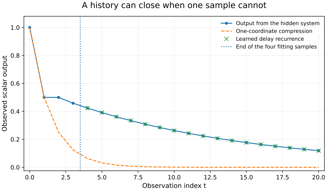
Output-only identification in the declared rational example. Four observations determine the delay recurrence. Later outputs are calculated independently from the hidden system. The one-coordinate compression omits the return path. This is a mathematical example, not a task-suite score.

View full-size figure (new tab)

Source and conversion record

Source SHA-256: 0173ab16e349b8778dc66f60f59820f40f800cff75e2223de07dcc1a84af18ff

Unsupported prose commands stop the build. The mathematical expression sequence is checked against the source, with manuscript macros expanded for display.

Conversion records

Notation in Large Signal Model

Look up a symbol without leaving this chapter. Select text before opening help to search for it.

Search this work’s notation.

    Symbols can have different meanings in different passages. Read each result in its own context.

    Open the full notation index