
9 A checked realization bridge for proof fields
On this page · Permalink · Source line 661
The ambient interpretation can be made into a mathematical construction rather than left as an analogy. The important step is to specify what a local realization means. A node label may describe an arbitrary mathematical sentence, but a Boolean value attached to that node does not automatically evaluate that sentence. In this section it records membership in a set closed under the declared certified rules. This restricted interpretation has an exact soundness and completeness theorem. An interpretation in actual mathematical propositions is a separate contract.
9.1 The declared rule system and its models
On this page · Permalink · Source line 667
Fix a node set \(V\), a set \(L\subseteq V\) of admissible leaves, and a set \(J\) of justifications. A justification \(j\) has a premise set \(A_j\), a conclusion \(c_j\), and a certification predicate. Define its support by
A set \(X\subseteq V\) is a model of the declared field when \(L\subseteq X\) and, for every certified \(j\),
Each justification is one implication with conjunctive premises. Alternative justifications remain separate implications. Uncertified attempts and failed-route annotations do not contribute a deduction rule merely by appearing in the archive.
Let \(\operatorname{Der}_F\) be the inductively generated set obtained from the leaves by certified rules. For a finite field, repeated forward closure computes this set. It is not necessary to enumerate all valuations to perform that computation.
Every declared field of this positive-implication form has a model: the full set \(V\). It contains every leaf and every rule conclusion. Nonexistence in the following extension problems therefore concerns prescribed local values or additional preservation requirements, not this unrestricted model space. This does not make every node derivable. Derivability is membership in the least model, not membership in some model.
Theorem 9.1: Soundness and relative completeness
For every node \(v\),
If \(v\) is not derivable, \(\operatorname{Der}_F\) itself is a model omitting \(v\).
Proof
Every model contains the leaves. Induction on a derivation shows that it contains the conclusion of every certified application whose premises have already been derived. Thus every model contains \(\operatorname{Der}_F\). Conversely, the inductive constructors show that \(\operatorname{Der}_F\) contains the leaves and is closed under every certified rule. It is therefore a model. Applying the universal condition to this particular model proves the reverse implication, and the same model gives the stated countermodel.
This is relative completeness for the declared rule system, not completeness of arbitrary mathematical proof search. A missing theorem may simply require a rule or a lemma absent from the field. A failed search can therefore produce a useful countermodel to a proposed finite inference architecture without disproving the mathematical target.
For an intended interpretation \(\mu:V\to\mathrm{Prop}\), the transfer to mathematical truth has explicit hypotheses: every leaf must satisfy \(\mu\), and every certified rule must preserve \(\mu\) from all its premises to its conclusion. Under those hypotheses, induction gives \(v\in\operatorname{Der}_F\Rightarrow\mu(v)\). Lean checks this statement as ProofPath.Field.semantic_soundness. It does not infer those hypotheses from a JSON certification flag.
9.2 From patches to a contravariant view system
On this page · Permalink · Source line 702
For a patch \(U\subseteq V\), let \(\mathcal M_F(U)\) consist of subsets \(X_U\subseteq U\) which contain \(L\cap U\) and obey every certified rule whose entire support lies in \(U\). If \(U\subseteq W\), define
This map is well defined. A rule supported in \(U\) is also supported in \(W\), and its conclusion remains in \(U\). The restriction therefore preserves both the local leaves and the local implication conditions.
Proposition 9.2: The proof-field view laws
The restriction maps satisfy
Consequently \(U\mapsto\mathcal M_F(U)\) is a contravariant set-valued view system on the inclusion order of patches.
Proof
Both laws are the corresponding intersection identities. For the second, \((X\cap W)\cap U=X\cap U\) because \(U\subseteq W\). The values outside a patch are absent, or equivalently normalized to false in the Lean representation. There are no additional hidden coordinates.
The strict Komorebi realization is now an actual set of coherent local models,
There is an explicit bijection
Its inverse evaluates a coherent family at the full patch \(V\). Coherence shows that every other component is precisely the restriction of that value. The Lean declaration ProofPath.Field.modelEquivSections constructs this equivalence, using ViewDiagram and the actual local restriction maps.
The full-patch equivalence identifies the ambient construction. It does not prove that arbitrary prescribed proper-patch data extend: the full patch already contains the global problem. Extension from smaller views is the distinct content of the following theorem.
Visual study 01: The bridge is a restriction map
On this page · Permalink · Source line 739
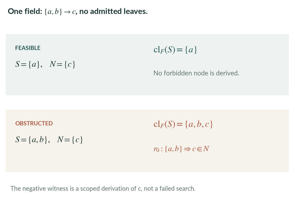
For one certified rule \(\{a,b\}\to c\) and no admissible leaves (\(L=\varnothing\)), there are seven global Boolean rule models. Only \((1,1,0)\) violates the implication. On either two-node patch below, the complete support is absent, so all four local valuations are admissible.
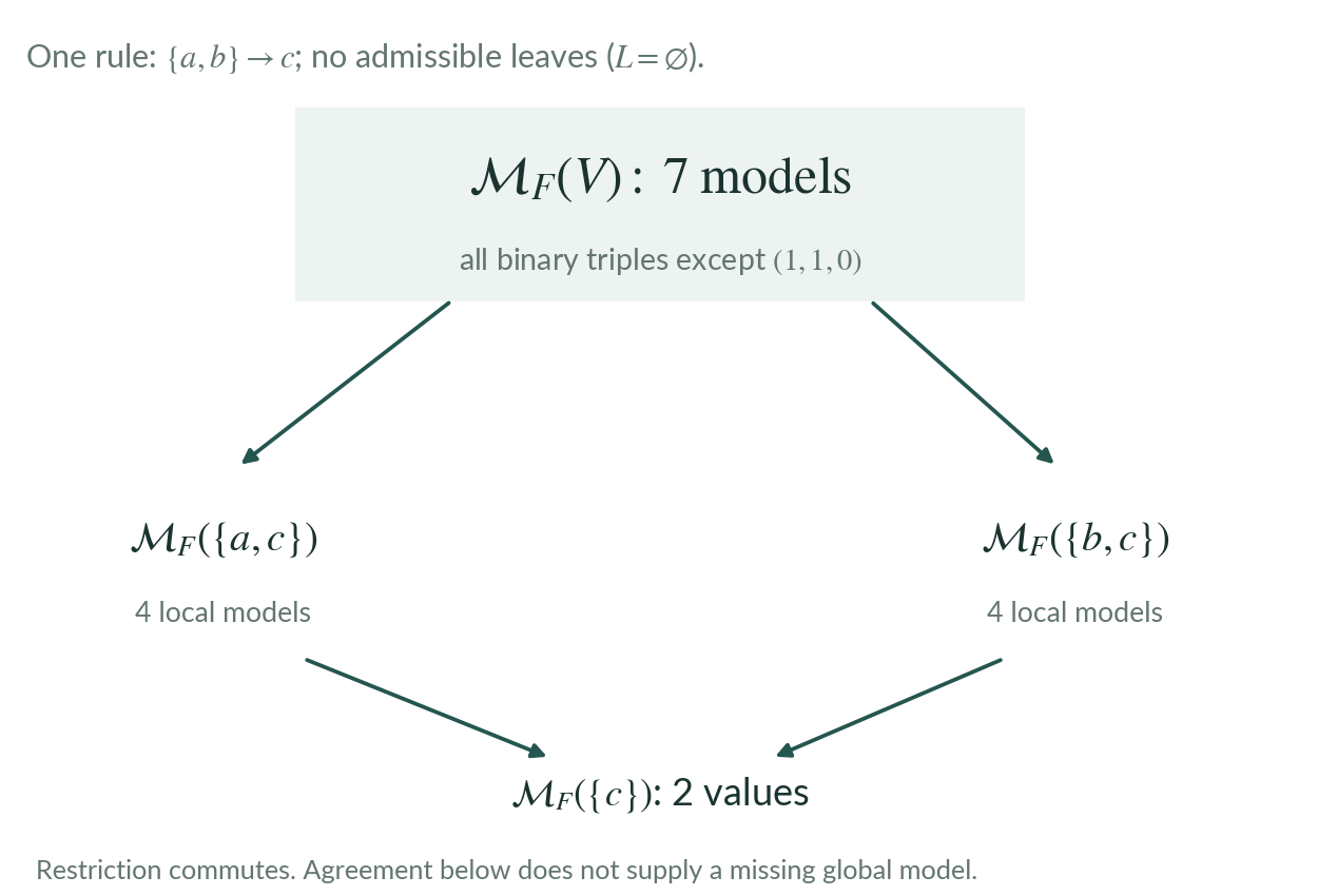
What the diagram establishes It displays the contravariant view construction and the consistency of restriction. The full-patch equivalence identifies global rule models with their coherent families of restrictions.
What the diagram does not establish A pair of matching proper-patch models need not be in the image of a global model. That extension question is controlled by the support of the rule, as the next study shows.
9.3 The correct coverage condition is a whole support
On this page · Permalink · Source line 756
Let \((U_i)_{i\in I}\) cover the nodes. A family \(X_i\in\mathcal M_F(U_i)\) is matching when
This equality includes agreement about false values, not merely common true values.
Theorem 9.3: Whole-support gluing
Suppose every certified justification has its whole support in some patch:
Then every matching family \((X_i)\) has a unique global field model \(X\) satisfying \(X\cap U_i=X_i\) for all \(i\).
Proof
Set \(X=\bigcup_iX_i\). Matching and node coverage imply \(X\cap U_i=X_i\). A leaf belongs to some patch and hence to its local model, so \(L\subseteq X\). Consider a certified rule whose premises belong to \(X\). Choose a patch containing its entire support. Matching implies that every premise is true in that patch's local model, whose rule condition forces the conclusion. Hence \(X\) obeys all certified rules. Any other global model with the specified restrictions agrees with \(X\) at every node because the patches cover the nodes. This proves uniqueness.
Example 9.4: Pairwise dependencies do not suffice
Take nodes \(a,b,c\), no admissible leaves (\(L=\varnothing\)), and one certified rule
Use patches \(U_0=\{a,c\}\) and \(U_1=\{b,c\}\). The local valuations \(X_0=\{a\}\) and \(X_1=\{b\}\) agree on their overlap: both assign false to \(c\). Both are local models, since neither patch contains the full rule support. They cover every node and both pairwise premise-to-conclusion dependencies. Nevertheless, a global model realizing them would contain \(a,b\) and omit \(c\), contradicting the rule. Thus replacing a conjunctive hyperedge by unrelated pairwise checks can lose precisely the constraint that matters.
The example is kernel checked in ProofPath.Examples. It does not contradict the earlier arrow-cover theorem. That theorem applies to a problem already specified by binary restriction equations. A conjunctive proof rule is a different constraint until a correct representation of its whole support has been supplied. The full support may be redundant in particular fields, so the theorem gives a sufficient cover condition rather than a necessary one for every individual diagram. Section 9.9 gives an exact entailment criterion for those redundancies.
The Python class ProofFieldViews implements these definitions. It freezes the rule and leaf contents at construction, restricts local valuations by literal intersection, checks support coverage before gluing, and can form a finite intersection-closed diagram for FiniteViewSystem. Local enumeration has explicit size limits. Forward closure and declared-field countermodels do not require that enumeration.
Visual study 02: Agreement can hide a missing rule
On this page · Permalink · Source line 791
Keep the same rule and choose the local data \(X_0=\{a\}\) on \(U_0=\{a,c\}\) and \(X_1=\{b\}\) on \(U_1=\{b,c\}\). Both local models assign false to their shared coordinate \(c\). They match exactly, yet their only assembled valuation violates the global rule.
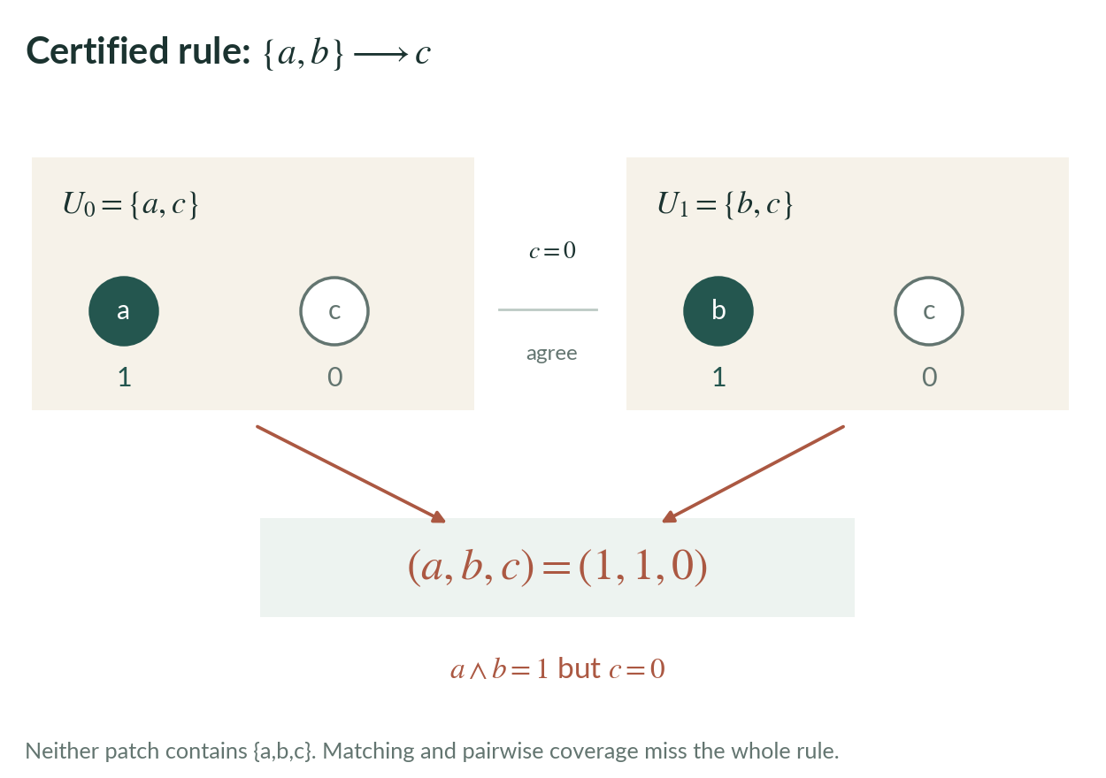
The successful gluing argument A patch containing the entire support \(\{a,b,c\}\) must enforce the conjunctive rule. If all local models match and every certified support occurs in a patch, their union obeys every rule. Node coverage then gives uniqueness. This is the content of Theorem 9.3, not an inference from pairwise agreement alone.
The cover condition is sufficient for all matching data. It need not be necessary for an individual field whose other rules already make a support constraint redundant.
9.4 Protected realization over a field
On this page · Permalink · Source line 807
The exact binary model admits a general algebraic formulation. Let \(K\) be a field, let \(E,R,S\) be \(K\)-vector spaces, and let \(D:E\to R\) and \(p:E\to S\) be linear. The prescribed problem is to repair \(x\) while retaining \(p(x)\):
The admissible correction image is \(B=D(\ker p)\). The elementary correction equivalence gives feasibility exactly when \(Dx\in B\).
Theorem 9.5: A linear certificate alternative
The protected problem is infeasible if and only if there is a linear functional \(\lambda:R\to K\) satisfying
For a finite matrix \(M\) and right side \(b\), the corresponding alternative is
Proof
If \(Dx\notin B\), linear separation of a vector from a subspace gives a functional vanishing on \(B\) and nonzero at \(Dx\). One construction extends a basis of \(B\) by \(Dx\) and then to a basis of \(R\). Assign value zero to the basis of \(B\) and value one to \(Dx\), and extend linearly. Equivalently, normalize any separating functional by its nonzero value. Conversely, if \(y\) were feasible, then \(h=x-y\) would satisfy \(p(h)=0\) and \(Dh=Dx\), contradicting the displayed functional equations. For a matrix, take \(B\) to be its column image. In finite coordinates the separating functional is a row vector, giving the stated alternative.
The general existence proof is classical. It does not claim an efficient procedure for arbitrary infinite spaces. In the implemented binary case, Gaussian elimination constructs a row witness, and the witness is checked against the original matrix and right side. A positive solution and a normalized negative witness cannot both verify.
Visual study 03: An obstruction is a checkable equation
On this page · Permalink · Source line 837
In the binary example from data/bridge_examples.json, compatibility demands \(a+b=0\) while the protected observations require \(a=0\) and \(b=1\). The variable \(c\) is unconstrained. Its freedom cannot remove the incompatible requirement on the first two coordinates.
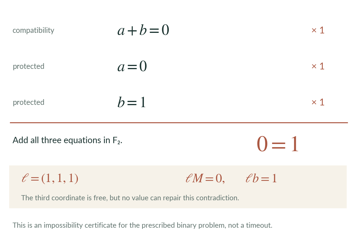
The exact system and witness can be inspected without trusting a search procedure:
If \(My=b\) had a solution, multiplying by \(\ell\) would give \(0=1\). This is a certificate for the declared protected problem. A search that merely stops supplies no comparable implication.
9.5 Counting what remains after an observation
On this page · Permalink · Source line 855
Let \(T:E\to R\) and \(Q:E\to W\) be linear, and fix a known point \(x_0\). Put
Translation \(h\mapsto x_0+h\) identifies \(H\) with \(\mathcal A\). The observation image is the translate \(Qx_0+Q(H)\), and the fiber above the attained value \(Qx_0\) is a translate of \(\ker Q_H\).
Theorem 9.6: Exact observation counts
Suppose \(K\) is a finite field of cardinality \(q\) and \(E\) is a finite-dimensional \(K\)-vector space. Set \(k=\dim_K H\) and \(r=\dim_K Q(H)\). Then
In particular the exact count identity is
Every attained observation fiber has the same size. For the uniform distribution on \(\mathcal A\), the observation removes exactly \(r\log_2q\) bits of uncertainty.
Proof
The two translation equivalences reduce the counts to finite vector spaces. Such a space of dimension \(d\) has \(q^d\) elements. Rank-nullity for \(Q_H\) gives \(\dim\ker Q_H+r=k\), proving the product identity and all the counts. An attained value can be treated by choosing a point attaining it as the base point. Equal fiber sizes imply a uniform observation distribution and a uniform conditional distribution on each fiber. The entropy difference is therefore \(\log_2(q^k)-\log_2(q^{k-r})=r\log_2q\).
Lean checks the translation equivalences, rank-nullity specialization, fiber cardinalities, and product identity in ProofPath.Protected, with the binary specialization in ProofPath.Binary. The logarithmic entropy interpretation is the written corollary above, not a newly compiled theorem about a Lean probability distribution. Uniformity is substantive. With a nonuniform prior, dimension alone does not determine Shannon information.
For the protected problem, set \(T=(D,p)\) and choose an actual feasible \(y_0\), so \(Ty_0=(0,px)\). This reduces its solution fiber to the theorem without changing the protected values. A concrete binary example has \(a+b+c=0\) and \(a=0\). Its two realizations are \((0,0,0)\) and \((0,1,1)\). Observing \(b\) has rank one on the ambiguity space and determines the remaining coordinate. Repeating the same observation in two output rows does not double the information.
Visual study 04: Ask what an observation distinguishes
On this page · Permalink · Source line 890
Return to the two vertices \(000\) and \(011\) from the opening cube. The ambiguity space is the span of \(011\). Reading the protected coordinate \(a\) repeats known information. Reading \(b\) separates the two points. Reading \(b\) twice creates two output rows but no additional distinction.
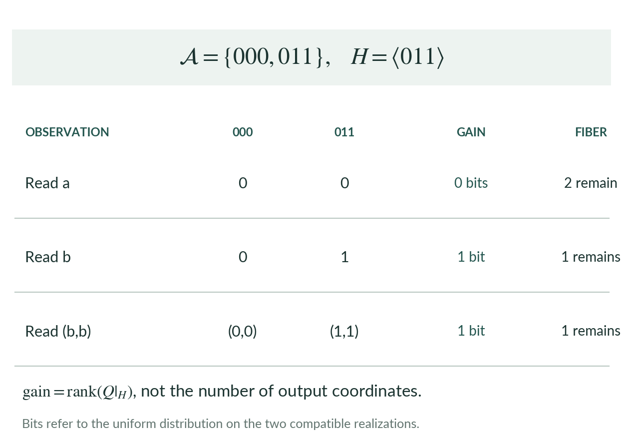
For example, the repeated observation has matrix
Its two rows are identical. On \(H=\langle011\rangle\) it has rank one, so \(|\mathcal A|=2\), \(|Q(\mathcal A)|=2\), and every attained observation fiber has size one. These are count identities before they are interpreted probabilistically.
The general finite-field formula in Theorem 9.6 retains the same separation: \(q^k\) initial possibilities, \(q^r\) attained outcomes, and \(q^{k-r}\) realizations per outcome.
9.6 Executable witnesses and a native declaration export
On this page · Permalink · Source line 909
Four exact examples are regenerated from the Python implementation: a one-bit ambiguity, an incompatible protected assignment, a redundant observation, and a uniquely determined realization. The generator emits the original stacked matrices and right sides alongside the proposed solutions or row witnesses. It also emits Lean declarations which check those concrete equations and cardinalities by kernel reduction. A faulty generator cannot make a false displayed proposition pass merely by assigning a certification flag. The generator itself is not thereby verified for arbitrary inputs, and the correspondence between the supplied JSON input and its emitted Lean syntax remains an audited software boundary.
A separate native exporter reads five already compiled Lean declarations, extracts their direct type and proof-constant dependencies, and records the transitive axiom sets. Dependencies outside the selected roots are explicit external leaves. This yields an actual proof-field JSON record rather than a hand-authored imitation of one. The exported field is then loaded through the public Python importer, and its declared closure is checked to contain its roots.
The export has a deliberately narrow meaning. It is syntactic dependency data for selected declarations, not a reconstruction of the entire discovery process. It does not recover failed attempts, prove that every constant in a type was a historically essential idea, or formally verify the metaprogram that extracts the data. The mathematical proof-field bridge is checked independently of that metaprogram. Its semantic interpretation retains the explicit hypotheses in Theorem 9.1.
9.7 Verification scope and reproducibility
On this page · Permalink · Source line 917
The present release freshly builds eighteen production Lean modules in a new object directory. Each module is replayed through Lean's own kernel against the pinned imported environment. The nine dependency revisions and the compiler hash are checked before building. All explicit named source declarations receive an axiom audit against the declared whitelist. The thirteen preceding mathematical modules are unchanged. Five new modules add executable trace checking, finite witness completeness, a typed JSON codec, and checked exchange examples.
Ten deliberately invalid files test false conclusions, missing support, placeholders, invalid decoders, merged observations, forged or incomplete closures, and a Boolean used as a node index. A further file introduces an explicit false axiom. Lean correctly accepts a consequence relative to that axiom, while the release's separate axiom policy rejects the dependency. A missing import, unavailable decision procedure, or timeout does not count as a mathematical rejection.
The fresh record is in evidence/formal_1.8.0/. The older record remains separately identified. Kernel replay here is not an independent implementation of Lean and does not rebuild or replay the entire cached Mathlib library. Written proofs, general Lean statements, generated concrete examples, and Python tests remain different evidence categories. In particular, a sound mathematical algorithm does not make its Python implementation universally verified.
9.8 Protected extensions of the actual rule field
On this page · Permalink · Source line 925
The linear model is not the only setting in which an obstruction can be returned explicitly. The original rule field has its own constructive extension problem. A partial Boolean description records which nodes must belong to a model and which must remain absent. These are observations about the declared model, not assertions that the sentences attached to the nodes are true or false in an intended mathematical universe.
Fix the field \(F\), including its admitted leaves and certified rules. For a positive observation set \(S\subseteq V\), let
where \(F[S]\) is obtained by admitting \(L\cup S\) as leaves and changing nothing else. For a negative observation set \(N\subseteq V\), define
Positive and negative observations are both part of the preservation contract. Dropping the negative observations can turn an impossible request into a different, feasible problem.
Theorem 9.7: Least protected extension and a complete obstruction
The extension fiber is nonempty exactly when
When this condition holds, \(\operatorname{cl}_F(S)\) is its least member. More generally,
If no extension exists, some \(n\in N\) has a derivation from \(L\cup S\) using only the declared certified rules.
Proof
Induction on a derivation shows that every model containing \(S\) contains \(\operatorname{cl}_F(S)\). The inductive closure is itself a model and contains \(S\). If it avoids \(N\), it is therefore a permitted extension, and the preceding inclusion proves leastness. If it meets \(N\), every model containing \(S\) contains a forbidden node, so no extension is possible. The displayed classification follows from the same inclusions. A point of the nonempty intersection is exactly the conclusion of the stated forbidden-node derivation.
This describes an interval inside the family of rule models, not an arbitrary interval of the power set. Closure under the rules remains essential. Nor is the fiber generally an affine space. For the rule \(\{a,b\}\to c\), with no leaves, \(S=\varnothing\) and \(N=\{c\}\), the allowed models are precisely \(\varnothing\), \(\{a\}\), and \(\{b\}\). There are three, not a power of two. The rank and entropy formulas for vector spaces cannot be imported into this model without additional structure.
Corollary 9.8: Exact extension of a partial valuation
Let \(S\subseteq U\subseteq V\). A global model whose true nodes on \(U\) are exactly \(S\) exists if and only if
Proof
Set \(N=U\setminus S\). Closure always contains \(S\), so avoiding \(N\) is equivalent to the displayed equality. Apply Theorem 9.7.
In particular, the test works for partial data that already violate a local rule. It need not assume local consistency and then hide that failure in a precondition. A contradictory observation can be exposed as a specific forbidden consequence.
Proposition 9.9: Staged closure and persistent obstructions
For positive sets \(S,T\),
If \(S\subseteq S'\) and \(N\subseteq N'\), then \(\operatorname{Ext}_F(S',N')\subseteq\operatorname{Ext}_F(S,N)\). Consequently an infeasible request stays infeasible under those additions, while the field and the meaning of its rules remain fixed.
Proof
Closure is extensive, monotone, and idempotent because it is the least model containing its seed. The model \(\operatorname{cl}_F(S\cup T)\) contains \(\operatorname{cl}_F(S)\) and \(T\), giving one inclusion in the first equation. Extensivity gives \(S\cup T\subseteq\operatorname{cl}_F(S)\cup T\), and monotonicity gives the other. A model satisfying the larger positive and negative prescriptions also satisfies the smaller ones. The last conclusion follows by inclusion of the extension fibers.
The module ProofPath.Extension checks these statements on the existing Field type. The Python module extension.py uses the same ProofFieldViews snapshot as the local-model construction. It computes closure by forward rule scans and records each newly derived node. At most \(|V|\) successful insertions occur. If a forbidden node is reached, a causal subtrace is extracted. It need not be the shortest or cheapest refutation.
The independent result checker replays that trace and checks that the recorded closure is closed under every rule. Derivability of every recorded node and closure of the recorded set together establish leastness. A negative witness only needs a valid derivation of one forbidden node. Its replay permits a previously derived node to have become an admitted observation, so the same witness can remain valid after positive data are strengthened. The checker does not call the producer, and a timeout is never returned as an obstruction.
9.9 Semantic covers rather than only syntactic covers
On this page · Permalink · Source line 1001
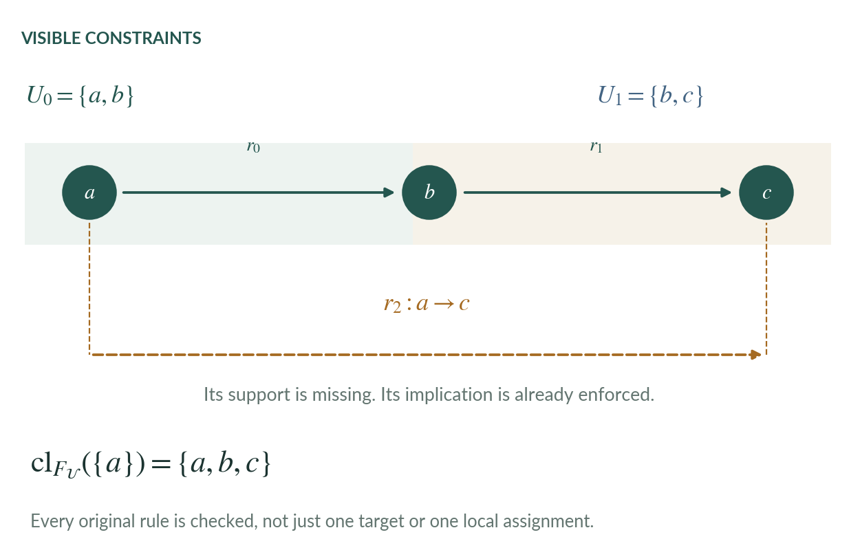
Whole-support coverage is easy to inspect and is sufficient for gluing. It can nevertheless be unnecessarily strong. Suppose \(F\) contains \(a\to b\), \(b\to c\), and \(a\to c\), with patches \(\{a,b\}\) and \(\{b,c\}\). The last support \(\{a,c\}\) is absent from both patches. Yet the first two visible rules already imply the last rule. Requiring another patch would duplicate information rather than restore a missing constraint.
Let \(\mathcal U=(U_i)_i\) cover every node. Define \(F_{\mathcal U}\) to have the same nodes and leaves as \(F\) but only those certified rules whose entire support lies in some \(U_i\). The distinction between the two fields is explicit. We call the cover semantically sufficient for the declared rules when
The word semantic here refers to the Boolean rule-model semantics of Section 9, not to an automatic interpretation of node labels as arbitrary mathematical truths.
Theorem 9.10: Exact criterion for universal gluing
Under node coverage, the following conditions are equivalent:
Every matching family of local \(F\)-models on the patches has a unique global \(F\)-model extending it.
Every model of \(F_{\mathcal U}\) is a model of \(F\).
Condition (SC) holds.
For every positive seed \(S\), \(\operatorname{cl}_{F_{\mathcal U}}(S)=\operatorname{cl}_F(S)\).
Whole-support coverage implies these conditions, but the converse need not hold.
Proof
A matching family assembles uniquely to a subset \(X\subseteq V\) because the patches cover all nodes and agree on their common coordinates. Its local rule conditions say exactly that \(X\) is a model of \(F_{\mathcal U}\). Conversely, a model of \(F_{\mathcal U}\) restricts to an \(F\)-model on every patch: every original rule supported in that patch is among the retained rules. Those restrictions match. Thus (i) and (ii) are equivalent, and uniqueness follows from node coverage.
Assume (ii) and fix a certified rule \(j\). The set \(\operatorname{cl}_{F_{\mathcal U}}(A_j)\) is a model of \(F_{\mathcal U}\) containing all of \(A_j\). By (ii) it obeys the original rule and contains \(c_j\), proving (iii). Conversely, if \(X\) is a model of \(F_{\mathcal U}\) containing \(A_j\), leastness gives \(\operatorname{cl}_{F_{\mathcal U}}(A_j)\subseteq X\). Condition (iii) therefore forces \(c_j\in X\). Every original rule is satisfied, which proves (ii).
Under (ii) the two fields have exactly the same models, since every \(F\)-model already obeys the retained rules. Their least models containing any seed are equal, giving (iv). If (iv) holds, apply it to \(A_j\). The conclusion \(c_j\) lies in \(\operatorname{cl}_F(A_j)\) by the original rule, so it lies in the retained closure as required by (iii). Finally, whole-support coverage retains every certified rule. The three-rule example above proves that this condition is not necessary.
There is a constructive negative result as well. If (SC) fails for \(j\), let
Then \(A_j\subseteq X\) and \(c_j\notin X\). The restrictions \(X\cap U_i\) are matching local \(F\)-models, but their only assembled subset violates the original rule. They are a checkable obstruction to universal gluing for this cover. They do not show that every matching family on the cover fails.
The module ProofPath.SemanticCover proves the criterion, including its connection to the actual Local, Matching, and gluedValue constructions. It is not a replacement field chosen only to have a convenient name. The Python producer returns a derivation of each original conclusion from its premises using only visible rules, or the countermodel just described. The verifier replays the positive derivations or checks the negative valuation directly. A new glue_semantic operation requires the positive certificate. The older glue method retains its simpler whole-support contract.
Visual study 05: A missing support can be redundant
On this page · Permalink · Source line 1041
The patches \(U_0=\{a,b\}\) and \(U_1=\{b,c\}\) do not contain the support of \(a\to c\). Their visible rules \(a\to b\) and \(b\to c\) nevertheless provide a certified derivation of that implication. Compare this with the missing conjunctive support in Figure 9: neither visible patch there provides a substitute for \(\{a,b\}\to c\).
Preserve the constraint, not necessarily its original presentation
The cover is sufficient because its visible rules impose the same models as the full field. The criterion checks every original rule, not just the target of one successful example.
For a finite field, one closure computation per original rule is enough to produce the positive certificates or expose a failed entailment. This avoids enumerating all local valuations or all matching families. The implementation uses repeated rule scans, so the release does not claim the indexed linear-time bound for its code. Its output certificates can be verified without trusting that search procedure.
9.10 Typed transport of derivations and obstructions
On this page · Permalink · Source line 1055
A change of proof-field representation needs more than a map of node names. Let \(F\) and \(G\) be declared fields. A rule transport consists of a node map \(f:V_F\to V_G\) and a rule map \(h:J_F\to J_G\) satisfying
The premise inclusion points in the direction needed for executing the translated step. The mapped target rule may need fewer premises, but it must not introduce a new premise unsupported by the source step. This is a sufficient, deliberately concrete transport interface. A more general translation could map one rule to an entire derivation.
Theorem 9.11: Compositional rule transport
Rule transports admit identities and associative composition. A transport \((f,h):F\to G\) sends every derivation of \(v\) in \(F\) to a derivation of \(f(v)\) in \(G\). Every \(G\)-model pulls back along \(f\) to an \(F\)-model. In particular,
An obstruction in the source extension problem therefore implies an obstruction in the target extension problem with the mapped observations.
Proof
Identity maps meet each displayed condition. For two composable transports, compose the node and rule maps. Applying the second map to the first premise inclusion and then using the second inclusion proves the composite premise condition. The conclusion and leaf conditions also compose. Function composition gives the identity and associativity laws.
Proceed by induction on a source derivation. A source leaf maps to a target leaf. For a rule step, every premise of the target rule is the image of a source premise, so the induction hypotheses supply all the required target premises. Certification and the conclusion equation then give the translated conclusion.
If \(Y\) is a target model, \(f^{-1}(Y)\) contains all source leaves. When it contains every premise of a source rule, \(Y\) contains every premise of the mapped rule and hence its conclusion. This proves the model pullback. Positive and negative observations pull back by their image definitions. If a target extension existed while the source problem were infeasible, its pullback would contradict that infeasibility.
Positive seeds can be added before transport. The same rule transport sends \(F[S]\) to \(G[f(S)]\), and hence
A forbidden source consequence \(n\in N\cap\operatorname{cl}_F(S)\) maps to the explicit forbidden consequence \(f(n)\in f(N)\cap\operatorname{cl}_G(f(S))\). The formal development checks this witness map, not only the existence statement obtained by contraposition.
Example 9.12: Why transport is not an equivalence
Let the source have nodes \(a,b\), no leaves, and no rules. The request \(a\) true and \(b\) false is feasible. Map both nodes to one target node \(u\), again with no leaves or rules. This is a rule transport, but the image request requires \(u\) both true and false and is infeasible. Thus source feasibility need not imply target feasibility, and target infeasibility need not imply source infeasibility.
ProofPath.RuleTransport checks these laws for actual derivations, and ProofPath.ExtensionExamples checks the collapse. The transported conclusion is true under an intended interpretation only if the target leaves and rules are sound. Renaming alone does not provide that contract.
9.11 Executable certificates for the declared closure
On this page · Permalink · Source line 1101
A mathematical characterization of closure is not yet a correctness theorem for the program that checks a certificate. The next construction closes that boundary for an explicit Lean checker. It uses the existing Field and seeded-closure definitions, rather than replacing their meaning by the output of an algorithm.
Definition 9.13: Finite indexed problem and trace
An indexed problem \(P\) specifies a finite address space \(V_n=\{0,\ldots,n-1\}\), admitted leaves \(L\), a list of certified rules, positive observations \(S\), and forbidden nodes \(N\). A rule at address \(j\) has a finite premise list \(A_j\) and conclusion \(b_j\). Two identical rows may have different rule addresses. Every listed node must belong to \(V_n\). Node lists are individually duplicate free, but \(L\), \(S\), and \(N\) need not be disjoint.
A trace \(\sigma=(j_1,\ldots,j_k)\) is a list of rule addresses. Replay begins with the list \(K_0=L\mathbin{+\!+}S\). It rejects an unknown rule address or a step whose premises are not all known. Otherwise it adds the conclusion. Strict replay additionally requires the conclusion to be new. Causal replay permits a conclusion already known. Lists are compared by membership when they represent sets.
Only rows declared certified enter this indexed rule list. The finite checker does not infer certification from a claim's label, its position in a document, or an author's confidence. An adapter that selects these rows must preserve the intended field and its assumptions.
Theorem 9.14: Replay preserves derivability and composes
Suppose every member of \(K\) belongs to \(\operatorname{cl}_F(S)\). If either replay mode accepts a trace starting from \(K\) and returns \(K'\), then
For a fixed replay mode, replaying \(\sigma\mathbin{+\!+}\tau\) is the same as replaying \(\sigma\) and then replaying \(\tau\) from the returned state. Failure at either stage propagates to the concatenated execution.
Proof
Induct on the trace. The empty trace returns the initial state. For a nonempty trace, a successful first step identifies a certified rule whose premises are already derivable. Closure under that rule proves its conclusion derivable. Adding the conclusion preserves all previously known nodes, and the induction hypothesis applies to the remaining trace. The stricter novelty test can reject a step but cannot invalidate this argument for an accepted one. The composition identity follows by the same induction, with the lookup and enabling tests taking the same branch on both sides.
The functions replay, enabled, and lookup are executable definitions. The formal theorems replay_sound, replay_extensive, and replay_append concern those definitions themselves. They are not specifications assumed of an otherwise unchecked replay routine.
Theorem 9.15: Acceptance identifies the least seeded model
A complete-closure certificate consists of a strict trace \(\sigma\) and a reported node list \(K\). The checker accepts precisely when replay succeeds, its output has the same members as \(K\), and \(K\) contains the admitted leaves and satisfies every declared rule. Acceptance implies
Here equality means equality of the represented sets, not equality of list order.
Proof
Theorem 9.14 gives \(K\subseteq\operatorname{cl}_F(S)\) because every initial node is an admitted leaf or a positive observation. Extensivity of replay ensures that \(K\) contains \(S\). The final closedness test makes \(K\) an \(F\)-model, so leastness of seeded closure gives the reverse inclusion. Both tests are needed: replay provides derivability, while the model test provides saturation under rules not used in the trace.
The connection to the prior theory is exact. In Lean, closed_iff_model identifies the Boolean rule check with the existing Field.Model predicate, and checkClosure_exact proves the displayed equality with Field.closure. For a valid indexed problem, valid_closure_bounded proves that every member of that closure has an address below \(n\). Thus totalizing rule lookup in the abstract Field cannot introduce a conclusion at an unnamed address: only successful lookups are certified.
Logical meaning remains a separate, explicit hypothesis. If an interpretation \(\mu:V_n\to\mathrm{Prop}\) satisfies the admitted leaves and rules, and every observation in \(S\) is true under \(\mu\), then every member of an accepted closure is true under \(\mu\). This follows by applying the prior model-soundness theorem to the derived nodes. Acceptance does not establish the truth of arbitrarily attached sentence labels.
9.12 Finite witnesses for forbidden consequences
On this page · Permalink · Source line 1145
Definition 9.16: Checked forbidden-node witness
A witness is a pair \((v,\tau)\), consisting of a target address and a causal trace. Its checker accepts when replay from \(L\cup S\) succeeds, the returned state contains \(v\), and \(v\in N\).
Theorem 9.17: Sound and complete obstruction witnesses
For the finite-premise indexed rule field,
The statement does not require the dependency graph to be acyclic.
Proof
An accepted witness derives a node in \(N\). Every model containing \(L\cup S\) contains that node, so no protected extension exists.
Conversely, Theorem 9.7 gives a forbidden node with an inductive derivation. Every such derivation has a finite causal trace. For an admitted leaf or observation, the empty trace suffices. For a rule application, obtain a trace for each of its finitely many premises by induction, concatenate those traces, and append the rule address. Previously derived nodes are never removed. A trace valid from one known set remains valid from a larger known set in causal mode, so the premise traces remain valid when concatenated. Repeated conclusions are allowed, including when an earlier premise trace already established one. The resulting trace derives the forbidden node and is accepted.
This proof explains the two replay modes. A causal witness can be reused after stronger positive observations make one of its intermediate conclusions already known. Requiring novelty at that point would reject a sound explanation. A complete-closure trace instead records fresh insertions and uses a separate final saturation test. The two contracts should not be conflated.
The Lean development proves trace weakening, strict-to-causal replay, finite premise-trace assembly, and derivation_has_trace before proving witness_exists_iff_infeasible. Witness existence is not a claim that a particular search procedure finds the shortest trace, nor is it a bound on the time taken by a Python producer.
Visual study 06: Why replay and closedness are both necessary
On this page · Permalink · Source line 1176
Take \(V_4=\{0,1,2,3\}\), \(L=\{0\}\), \(S=\varnothing\), and the two rules \(r_0:0\to1\) and \(r_1:1\to2\). The least closure is \(\{0,1,2\}\). Node \(3\) has no derivation from these inputs.
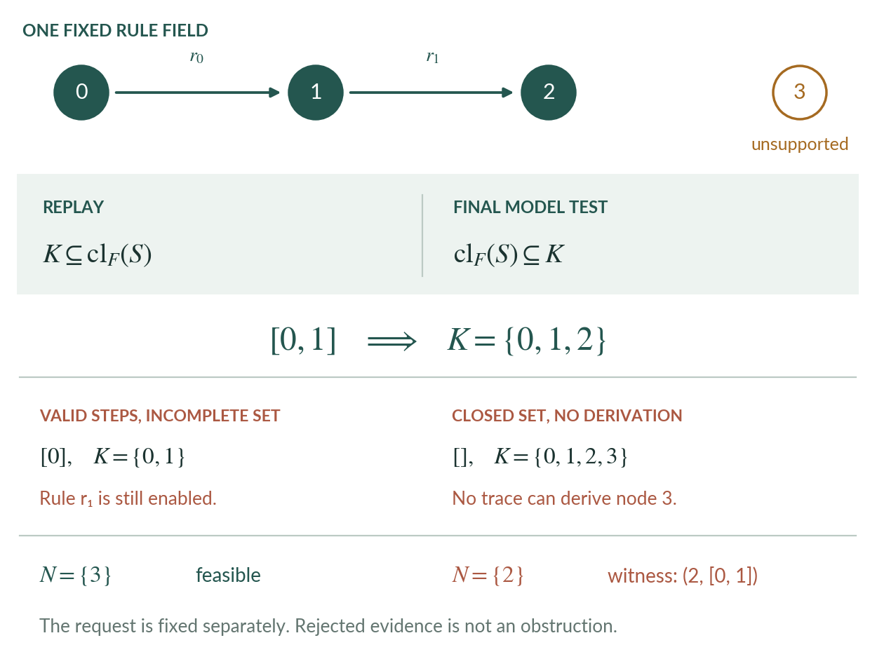
The trace \([0]\) derives exactly \(\{0,1\}\) but leaves \(r_1\) enabled with its conclusion absent. It is a valid partial derivation, not a complete closure. Conversely, \(\{0,1,2,3\}\) is closed under both rules, but replay cannot establish its unsupported node \(3\). A model need not be the least model.
With \(N=\{3\}\), the exact closure gives a positive result. With \(N=\{2\}\), the same closure supports a negative result with witness \((2,[0,1])\). The second problem is not a different interpretation of the same request: its protected observations have changed. A checker must receive the fixed request separately from the proposed answer.
Corollary 9.18: Meaning of a complete result certificate
The complete result format contains a Boolean feasibility flag, a reported closure, a strict closure trace, and an optional forbidden-node witness. Both branches require the complete-closure check. A positive result additionally requires no obstruction witness and no forbidden node in the closure. A negative result requires an accepted obstruction witness. For every accepted result \(C\),
Proof
The complete-closure check proves the first equality. In the positive branch, the closure is a model containing \(S\) and avoiding \(N\), hence is an extension. In the negative branch, the witness excludes every extension by Theorem 9.17. Case analysis on the Boolean flag gives the equivalence.
A bare negative witness has its own checker and does not need a saturated closure. The complete result format asks for both because it promises both an exact closure and a feasibility verdict. Failure of either check means that this certificate was not accepted. It is not itself a refutation of the protected problem.
9.13 Typed exchange and the boundary of serialization
On this page · Permalink · Source line 1208
A certificate is useful outside its producer only when the receiving system knows exactly which data it checked. The exchange format therefore uses versioned positional arrays, exact nonnegative integer tokens, literal Booleans, and explicit rule addresses. Problem and certificate are separate records. The node address book and the selected certified-rule order remain associated with the originating proof-field snapshot.
At the JSON syntax-tree level, the problem has the shape
["proof-path/problem/1", node_count, leaves, rules, positive, negative]where each rule is [premises, conclusion]. The certificate has the shape
["proof-path/certificate/1", feasible, closure, trace, obstruction]where an obstruction is either null or [target, trace]. Array lengths and tags are exact. A Boolean is not an integer address, and the string "false" is not a Boolean verdict. Duplicate node entries are rejected by validity checks, while identical rule rows at different addresses remain distinguishable.
Theorem 9.19: Lossless encoding at the typed syntax boundary
Let \(e_P,d_P\) and \(e_C,d_C\) be the stated Lean encoders and partial decoders for problem and certificate records. For every typed problem \(P\) and certificate \(C\),
Consequently both encoders are injective on their typed domains. These identities do not require the encoded record to pass the separate validity checks.
Proof
The natural-number and Boolean constructors decode to their original values. Induction on a list proves the corresponding array round trip. The rule, witness, and optional-witness decoders then recover their components. Unfolding the exact-length record encoders and decoders gives the two identities. If two encoded records are equal, applying the decoder gives equal some values, hence equal original records.
Theorem 9.20: Accepted JSON records certify their decoded answer
Suppose the JSON checker accepts the separately supplied problem and certificate syntax trees. Then both decode to typed records \(P,C\), both pass their index and shape checks, and the decoded certificate satisfies the closure equality and feasibility equivalence of Corollary 9.18 for that decoded problem.
Proof
The executable checker rejects any failed decoding or validity check. In the remaining branch it calls the same complete result checker used in Corollary 9.18. Its acceptance therefore supplies that corollary's hypothesis. The round-trip identities additionally show that checking encoded typed records agrees with checking those records directly.
The general proof ends at Lean's Json syntax-tree interface. It does not prove the correctness of the standard text parser, printer, file system, Python interpreter, or name-to-index adapter. The command-line reader is executed on actual canonical bytes and compared with an independent finite model oracle. That conformance test complements the formal theorem without extending its quantified scope.
Canonical standalone files use compact ASCII JSON with an optional final newline. Decimal or exponent spellings, alternative internal whitespace, extra fields, and duplicate object-key constructions are outside this exchange contract. The format uses no objects. Resource limits are explicit operational rejections, not evidence that a protected realization is impossible. The encoder's injectivity is a statement about retained data, not a collision-freedom claim for a later cryptographic hash.
The package supplies actual named-field exports, a separate indexed Python checker, the Lean text adapter, and generated Lean fixtures for six concrete exchanges. Their role is to test the entire executed route as well as its proved core. The original named proof fields remain finite and acyclic. Cyclic examples belong to the lower-level indexed checker and show that its soundness theorem does not depend on topological sorting. An unseeded cycle supplies no finite derivation merely by referring to itself.