
Quantum phase, measurement, and information loss
An extended hand-worked example · Komorebi P.
Start with a two-component state whose amplitudes are known exactly. Change its relative phase, measure it in three different settings, and reconstruct its density matrix. Then remove the coherence and identify precisely which questions can still be answered. Continue through amplitude damping, the collection's modulus-12 interference example, and a three-qubit recovery code.
Run the phase comparison · Run partial dephasing and tomography · Run the modulus-12 phase experiment · Read the exact Python program · Download source and results
This is a standard finite quantum-mechanics calculation presented through the collection's packet and recovery language. All displayed probabilities are exact ensemble probabilities. Repeated experimental measurements would estimate them; a single measurement does not reveal a density matrix.
1. Declare the state and the coordinates
Use the orthonormal basis \(\{|0\rangle,|1\rangle\}\) of \(\mathbb C^2\). For a phase \(z\in\mathbb C\) with \(|z|=1\), let
\[
|\psi_z\rangle=\frac35|0\rangle+\frac45z|1\rangle,
\qquad
\rho_z=|\psi_z\rangle\langle\psi_z|
=\begin{pmatrix}
9/25&(12/25)\overline z\\
(12/25)z&16/25
\end{pmatrix}.
\]
The squared norm is \(9/25+16/25=1\). Consequently \(\rho_z^*=\rho_z\), \(\operatorname{tr}\rho_z=1\), and \(\rho_z^2=\rho_z\). Positivity follows directly from \(v^*\rho_zv=|\langle\psi_z,v\rangle|^2\ge0\). The purity \(\operatorname{tr}(\rho_z^2)\) is one.
The two coordinate projectors are \(P_0=\operatorname{diag}(1,0)\) and \(P_1=\operatorname{diag}(0,1)\). Their four density-matrix blocks are
\[
P_0\rho_zP_0=\frac9{25}|0\rangle\langle0|,
\quad P_1\rho_zP_1=\frac{16}{25}|1\rangle\langle1|,
\quad P_0\rho_zP_1=\frac{12}{25}\overline z|0\rangle\langle1|,
\quad P_1\rho_zP_0=(P_0\rho_zP_1)^*.
\]
The diagonal blocks contain the populations. The off-diagonal blocks contain the coherence between the two declared packets. Adding all four blocks reconstructs the state exactly. A global phase multiplying both amplitudes cancels in \(\rho_z\); the relative phase \(z\) remains.
2. Change the measurement setting
Write a general qubit density matrix as \(\rho=\begin{pmatrix}p&c\\\overline c&1-p\end{pmatrix}\). The Pauli observables and their plus-outcome projectors are
\[
X=\begin{pmatrix}0&1\\1&0\end{pmatrix},\quad
Y=\begin{pmatrix}0&-i\\i&0\end{pmatrix},\quad
Z=\begin{pmatrix}1&0\\0&-1\end{pmatrix},
\qquad E_{A,+}=\frac{I+A}{2}.
\]
For each setting \(A\in\{X,Y,Z\}\), the minus effect is \(I-E_{A,+}\). The Born rule gives
\[
\boxed{p_{X,+}=\frac12+\operatorname{Re}c,\quad
p_{Y,+}=\frac12-\operatorname{Im}c,\quad p_{Z,+}=p.}
\]
For our state, \(c=(12/25)\overline z\), so
\[
p_{X,+}=\frac12+\frac{12}{25}\operatorname{Re}z,
\qquad p_{Y,+}=\frac12+\frac{12}{25}\operatorname{Im}z,
\qquad p_{Z,+}=\frac9{25}.
\]
The sign in the Y formula matters: the upper-right entry is the conjugate of the lower-left entry. With the displayed convention, a positive imaginary part of \(z\) increases the Y-plus probability.
| Relative phase \(z\) | X-plus | Y-plus | Z-plus |
|---|---|---|---|
| \(1\) | \(49/50\) | \(1/2\) | \(9/25\) |
| \(i\) | \(1/2\) | \(49/50\) | \(9/25\) |
| \(-1\) | \(1/50\) | \(1/2\) | \(9/25\) |
| \(-i\) | \(1/2\) | \(1/50\) | \(9/25\) |
| \((3+4i)/5\) | \(197/250\) | \(221/250\) | \(9/25\) |
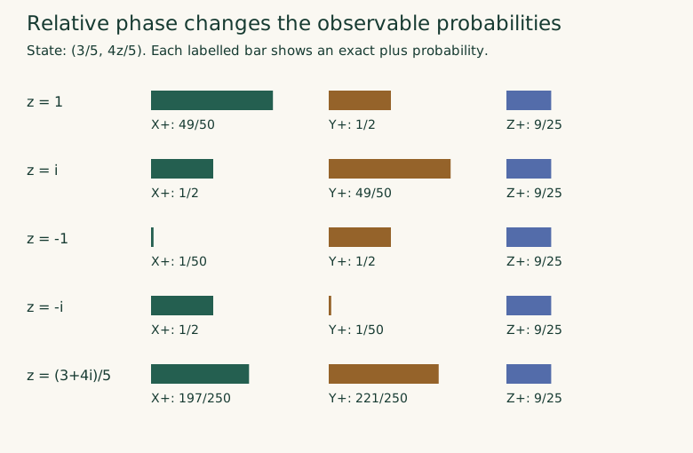
Figure 1. One state family measured in three settings. The Python program generates this diagram and its exact CSV. Bar widths use rounded drawing coordinates; their fraction labels and the table give the exact values.
The Hadamard matrix \(H=\frac1{\sqrt2}\begin{pmatrix}1&1\\1&-1\end{pmatrix}\) turns an X measurement into a coordinate measurement because \(H^*ZH=X\). Thus the coordinate probabilities of \(H|\psi_z\rangle\) are \((p_{X,+},1-p_{X,+})\). The factors of \(\sqrt2\) cancel when computing \(H\rho H^*\), allowing exact arithmetic in \(\mathbb Q(i)\) for all five phases above.
3. Forget a coordinate measurement outcome
A selective coordinate measurement returns outcome \(j\) with probability \(p_j\). Conditional on an outcome of nonzero probability, the state is \(P_j\rho P_j/p_j\). For this family these conditional states are \(P_0\) and \(P_1\).
If the outcome is discarded, the channel is
\[
\mathcal D(\rho)=P_0\rho P_0+P_1\rho P_1,
\qquad
\mathcal D(\rho_z)=\begin{pmatrix}9/25&0\\0&16/25\end{pmatrix}.
\]
The Kraus completeness relation is \(P_0^*P_0+P_1^*P_1=I\). The channel preserves trace and positivity, and \(\mathcal D^2=\mathcal D\). It deletes the two cross-packet blocks. Its output purity is
\[
\boxed{\operatorname{tr}(\mathcal D(\rho_z)^2)
=\left(\frac9{25}\right)^2+\left(\frac{16}{25}\right)^2
=\frac{337}{625}.}
\]
For every coordinate-diagonal effect \(E=\operatorname{diag}(e_0,e_1)\), with \(0\le e_j\le1\),
\[
\operatorname{tr}(E\rho_z)
=e_0\frac9{25}+e_1\frac{16}{25}
=\operatorname{tr}(E\mathcal D(\rho_z)).
\]
That measurement cannot detect the discarded coherence. An X or Y measurement can: after dephasing, both plus probabilities become \(1/2\).
This gives an exact recovery obstruction. The states \(\rho_1\) and \(\rho_i\) have the same dephased output, but their X-plus probabilities are \(49/50\) and \(1/2\). A function of that output alone cannot return both answers. Z probabilities remain recoverable from it.
4. Retain a controlled amount of coherence
Let \(0\le t\le1\) and define
\[
\mathcal D_t=t\,\operatorname{id}+(1-t)\mathcal D,
\qquad
\mathcal D_t(\rho)=\begin{pmatrix}p&tc\\t\overline c&1-p\end{pmatrix}.
\]
Here \(t\) is the retained coherence, rather than the probability of performing a measurement. An independent implementation is the random phase-flip channel
\[
\mathcal D_t(\rho)=\frac{1+t}{2}\rho+
\frac{1-t}{2}Z\rho Z.
\]
The weights are nonnegative and sum to one; the corresponding Kraus operators are \(\sqrt{(1+t)/2}\,I\) and \(\sqrt{(1-t)/2}\,Z\). Multiplication of the two off-diagonal entries verifies the formula directly. In particular, \(\mathcal D_s\mathcal D_t=\mathcal D_{st}\).
For the family \(\rho_z\), direct matrix multiplication gives
\[
\boxed{\operatorname{tr}(\mathcal D_t(\rho_z)^2)
=\frac{337+288t^2}{625}.}
\]
For a matrix \(A\), define \(\|A\|_{\mathrm{HS}}^2=\operatorname{tr}(A^*A)\). The lost part is entirely off diagonal, giving
\[
\|\rho_z-\mathcal D_t(\rho_z)\|_{\mathrm{HS}}^2
=\frac{288}{625}(1-t)^2.
\]
For \(z=1\), selected exact checkpoints are:
| Retained coherence \(t\) | X-plus | Y-plus | Purity |
|---|---|---|---|
| \(0\) | \(1/2\) | \(1/2\) | \(337/625\) |
| \(1/2\) | \(37/50\) | \(1/2\) | \(409/625\) |
| \(1\) | \(49/50\) | \(1/2\) | \(1\) |
The browser experiment plots nine rational values of \(t\) and exports their exact fractions.
5. Recover the density matrix from three settings
Solving the probability equations in section 2 gives
\[
\boxed{\rho=
\begin{pmatrix}
p_{Z,+}&p_{X,+}-\frac12+i(\frac12-p_{Y,+})\\
p_{X,+}-\frac12-i(\frac12-p_{Y,+})&1-p_{Z,+}
\end{pmatrix}.}
\]
For \(z=(3+4i)/5\), the measured triple \((197/250,221/250,9/25)\) reconstructs
\[
\rho=\begin{pmatrix}
9/25&(36-48i)/125\\
(36+48i)/125&16/25
\end{pmatrix}.
\]
These are three alternative measurement settings on identically prepared copies. They are not three simultaneous outcomes on one qubit. Arbitrary noisy triples also need not produce a positive matrix; the exact data here come from the stated density matrices.
If a known \(t>0\) was applied first, ideal tomography reconstructs \(\mathcal D_t(\rho)\), and division of its off-diagonal entries by \(t\) recovers the original entries algebraically. Measurement error in those entries is amplified by \(1/t\). At \(t=0\), division is impossible and the two-state obstruction in section 3 applies.
Write \(|+\rangle=(|0\rangle+|1\rangle)/\sqrt2\). This algebraic inverse on the channel's image is not a physical recovery channel on arbitrary input states. For example, at \(t=1/2\), doubling the coherence of \(|+\rangle\langle+|\) would give
\[
A=\begin{pmatrix}1/2&1\\1&1/2\end{pmatrix},
\qquad (1,-1)A(1,-1)^{\mathsf T}=-1<0.
\]
The output would fail positivity. This particular pure input is outside the image of \(\mathcal D_{1/2}\) on density matrices.
6. Operation order changes the answer
Use \(z=1\). Changing basis before dephasing gives
\[
\mathcal D(H\rho_1H^*)=
\begin{pmatrix}49/50&0\\0&1/50\end{pmatrix}.
\]
Dephasing before changing basis gives
\[
H\mathcal D(\rho_1)H^*=
\begin{pmatrix}1/2&-7/50\\-7/50&1/2\end{pmatrix}.
\]
A final coordinate measurement has outcome-0 probability \(49/50\) in the first experiment and \(1/2\) in the second. The difference is \(12/25\). Changing the measurement setting after the phase was removed cannot recover the original interference.
7. A coherent record can be uncomputed
Introduce a second qubit, initially \(|0\rangle\), and use system-first address order \(00,01,10,11\). A controlled-NOT from the system to the record sends
\[
|\psi_z\rangle|0\rangle\longmapsto
|\Omega_z\rangle=\frac35|00\rangle+\frac45z|11\rangle.
\]
The joint state remains pure and retains cross entries between addresses \(00\) and \(11\). Its reduced system state is \(\operatorname{tr}_{\mathrm{record}}|\Omega_z\rangle\langle\Omega_z| =\mathcal D(\rho_z)\). Partial trace ignores the record; it does not erase the joint coherence. If both qubits remain coherently accessible, applying the same controlled-NOT again returns \(|\psi_z\rangle|0\rangle\).
If the record has instead been measured in its coordinate basis and only the classical outcome is retained, the joint density matrix is
\[
\frac9{25}|00\rangle\langle00|
+\frac{16}{25}|11\rangle\langle11|.
\]
Applying controlled-NOT now produces \(\mathcal D(\rho_z)\otimes|0\rangle\langle0|\). The classical label tells us which branch occurred, but contains no relative phase. Restoring that phase would require coherent access to all relevant degrees of freedom carrying the record. Uncomputation of the two qubits alone no longer supplies it.
8. Refine the packets and see which coherence disappears
For a separate two-qubit example, use \(|\Phi^+\rangle=(|00\rangle+|11\rangle)/\sqrt2\). Its density matrix has four entries equal to \(1/2\), at \((00,00),(00,11),(11,00),(11,11)\).
The parity packets are
\[
P_{\mathrm{even}}=|00\rangle\langle00|+|11\rangle\langle11|,
\qquad
P_{\mathrm{odd}}=|01\rangle\langle01|+|10\rangle\langle10|.
\]
The state lies entirely in the even packet. Forgetting a parity-measurement outcome therefore leaves it unchanged, with purity one. Its coherence between \(00\) and \(11\) is within that packet.
Refine the measurement into four singleton-address projectors and forget their outcomes. Now the same coherence is between distinct packets and is deleted. The result is
\[
\frac12|00\rangle\langle00|+\frac12|11\rangle\langle11|,
\qquad \text{purity }\frac12.
\]
Declaring finer coordinates while retaining all matrix blocks is reversible. Performing the finer measurement and discarding its outcome is a different operation. This example makes the distinction explicit.
9. Amplitude damping transfers population as well as coherence
Paper VII's Kraus-transfer example uses amplitude damping. For \(0\le\gamma\le1\), its two Kraus operators are
\[
K_0=\begin{pmatrix}1&0\\0&\sqrt{1-\gamma}\end{pmatrix},
\qquad K_1=\begin{pmatrix}0&\sqrt\gamma\\0&0\end{pmatrix}.
\]
Their adjoint products sum to \(I\). Multiplying both branches gives
\[
\Phi_\gamma\!\begin{pmatrix}p&c\\\overline c&q\end{pmatrix}
=\begin{pmatrix}
p+\gamma q&\sqrt{1-\gamma}\,c\\
\sqrt{1-\gamma}\,\overline c&(1-\gamma)q
\end{pmatrix},\qquad p+q=1.
\]
The excited population \(q\) sends \(\gamma q\) to the ground packet. The two off-diagonal blocks are multiplied by \(\sqrt{1-\gamma}\). This differs from coordinate dephasing, which leaves both populations fixed.
Choose \(\gamma=9/25\), so the square roots are \(3/5\) and \(4/5\). For the original state with \(z=1\), every entry is rational:
\[
\Phi_{9/25}(\rho_1)=
\begin{pmatrix}369/625&48/125\\48/125&256/625\end{pmatrix}.
\]
The lost excited population is \((9/25)(16/25)=144/625\), exactly the increase in ground population. X-plus becomes \(221/250\); Z-plus becomes \(369/625\). The determinant and purity are
\[
\det\Phi_{9/25}(\rho_1)=\frac{36864}{390625},
\qquad
\operatorname{tr}(\Phi_{9/25}(\rho_1)^2)
=1-2\det\Phi_{9/25}(\rho_1)=\frac{316897}{390625}.
\]
Purity is not a universal measure of how much information a channel retains. The same channel sends \(I/2\), of purity \(1/2\), to \(\operatorname{diag}(17/25,8/25)\), of purity \(353/625>1/2\). At \(\gamma=1\), every input becomes \(|0\rangle\langle0|\), a pure state that contains no information about the input. The program checks the Kraus calculation at both endpoints and at \(\gamma=9/25\).
10. The collection's modulus-12 phase example
The Quantum and Circuits book contains a stronger version of the equal-histogram example. Its quantum arithmetic chapter uses the Ramanujan-sum vector
\[
c=(4,0,2,0,-2,0,-4,0,-2,0,2,0),\qquad
a=|c|=(4,0,2,0,2,0,4,0,2,0,2,0).
\]
Here \(c\) is a twelve-component vector, separate from the scalar off-diagonal entry used earlier. Both vectors have squared norm \(48\). The normalized states \(\psi=c/\sqrt{48}\) and \(\chi=a/\sqrt{48}\) have the same coordinate probabilities: \(1/3\) at addresses 0 and 6, \(1/12\) at addresses 2, 4, 8, and 10, and zero elsewhere. Nevertheless,
\[
\langle\psi,\chi\rangle
=\frac{16+4-4-16-4+4}{48}=0.
\]
Let \(U_{12}=\{1,5,7,11\}\), the labels coprime to twelve. Use the unitary Fourier convention \(F_{nk}=e^{2\pi i nk/12}/\sqrt{12}\), and let \(D\) select those four Fourier labels. The book's rational selector is
\[
P=FDF^*,\qquad P_{nm}=\frac{c((n-m)\bmod12)}{12}.
\]
Direct multiplication gives \(P^2=P=P^*\), \(Pc=c\), and \(Pa=0\). Thus a measurement of \(\{P,I-P\}\), equivalently applying \(F^*\) followed by selection of \(U_{12}\), accepts \(\psi\) with probability one and \(\chi\) with probability zero. Identical initial histograms can conceal perfectly distinguishable states. These are the book's QA13–QA14 calculations.
Vary the phase continuously
Let \(v_+\) retain the positive entries of \(c/\sqrt{48}\), and let \(v_-\) retain the absolute values of its negative entries. Their disjoint supports each have squared norm \(1/2\). For \(|z|=1\), define
\[
\chi_z=v_++zv_-
=\frac{1+z}{2}\chi+\frac{1-z}{2}\psi.
\]
Every member has the same coordinate histogram, while
\[
\boxed{\|P\chi_z\|^2=\frac{|1-z|^2}{4}
=\frac{1-\operatorname{Re}z}{2}.}
\]
For \(z=e^{i\theta}\), this is \(\sin^2(\theta/2)\), the book's QA19 phase-response formula. The endpoints \(z=1\) and \(z=-1\) are the unsigned and signed states.
Replacing signs is different from removing coherence
Complete coordinate dephasing of any member gives \(\rho_{\mathrm{diag}}=\operatorname{diag}(c(n)^2/48)\). Every diagonal entry of \(P\) is \(c(0)/12=1/3\), so
\[
\boxed{\operatorname{tr}(P\rho_{\mathrm{diag}})=\frac13.}
\]
The three cases are therefore distinct:
| Preparation | Selected probability |
|---|---|
| Signed coherent state \(\psi\) | \(1\) |
| Unsigned coherent state \(\chi\) | \(0\) |
| Either state after complete coordinate dephasing | \(1/3\) |
This is QA20 in the book. Replacing negative amplitudes by positive ones leaves a coherent state; it is not the dephasing channel. The book records QA19 and QA20 as prose results beyond its inherited Lean package. The new program and browser experiment check this finite example with exact rational projector arithmetic.
11. A syndrome can reveal an error without revealing the logical state
Paper VII's three-qubit bit-flip example encodes the same logical state as
\[
|\psi_L\rangle=\frac35|000\rangle+\frac45z|111\rangle.
\]
Write \(\rho_L=|\psi_L\rangle\langle\psi_L|\) for its density matrix.
Consider the error family \(E_0=I\), \(E_1=X\otimes I\otimes I\), \(E_2=I\otimes X\otimes I\), and \(E_3=I\otimes I\otimes X\). Each error sends the code to one of four mutually orthogonal packets:
| Error | Image of logical 0 | Image of logical 1 | Correction |
|---|---|---|---|
| \(I\) | 000 | 111 | \(I\) |
| First-bit flip | 100 | 011 | First-bit flip |
| Second-bit flip | 010 | 101 | Second-bit flip |
| Third-bit flip | 001 | 110 | Third-bit flip |
Let \(S_j\) project onto the pair in row \(j\). These packets cover all eight addresses, so \(\sum_j S_j=I\). A syndrome measurement uses these two-dimensional packets without distinguishing the two addresses inside one row. It preserves their logical coherence, including \(z\).
For a normalized noise channel \(\mathcal N(\rho_L)=\sum_j q_jE_j\rho_LE_j^*\), where \(q_j\ge0\) and \(\sum_jq_j=1\), choose recovery branches \(R_j=E_jS_j\). Their adjoint products sum to \(I\). Orthogonality of the four packets and \(E_j^2=I\) give
\[
\sum_jR_j\mathcal N(\rho_L)R_j^*=\rho_L.
\]
The outcome distribution is \((q_j)\), independent of the logical amplitudes and phase. A classical syndrome record can therefore identify which correctable error occurred without exposing the logical state. This is different from the coordinate record in section 7.
If the measurement instead resolves all eight individual addresses and discards its outcome, the logical off-diagonal entries disappear. Applying the same correction then returns the dephased logical state. Recovery depends on which measurement was performed.
This code corrects the stated family of single bit flips. Two flips can share a syndrome with a different single flip and produce a logical bit flip after correction. A physical phase flip can remain inside the code packet and alter the logical phase without being detected. The program checks both limitations, all four correctable branches, and their mixture with probabilities \((1/2,1/4,1/8,1/8)\).
Reproduce the calculation
Download the standalone program and run it with Python 3.10 or later. It uses only the standard library.
python -B quantum_phase_measurement.py
python -B quantum_phase_measurement.py --output quantum-results
Coordinate probabilities: 9/25, 16/25
X-plus, phase 1: 49/50; phase i: 1/2
Y-plus, phase 1: 1/2; phase i: 49/50
Purity: original 1; dephased 337/625; half coherence 409/625
Order witness, outcome 0: 49/50 versus 1/2
Coherent record: reversible; classical record: phase lost
Bell purity: parity packets 1; individual addresses 1/2
Damping: ground population 369/625; purity 316897/390625
Arithmetic selector: unsigned 0; signed 1; dephased 1/3
Syndrome recovery: four single-error branches preserve the logical state
PASS: 1917 exact cases
The suite covers 182 pure-state cases using rational circle parameters, 910 partial-channel cases, 182 coherent/classical record comparisons, and 10 fixed controls. The collection extensions add 546 damping cases, 15 arithmetic-projector cases, and 72 syndrome/recovery cases. The suite uses direct matrix products and independent random-unitary channel formulas. These finite checks accompany the hand derivations; they are not a proof about all quantum systems or a replay of the collection's Lean evidence.
Measurement settings CSV · Partial dephasing CSV · Exact results JSON · Amplitude damping CSV · Arithmetic phase CSV · Syndrome recovery CSV · Revision and SHA-256 source record
Papers, written proofs, and scope
Read the matching Paper VII chapters
| Topic | Illustrated chapter | Statement and proof |
|---|---|---|
| Which measurements detect coherence? | Measurements | Measurement invariance · Proof |
| What does a channel transfer? | Kraus channels and amplitude damping | Finite Kraus channel · Proof |
| When can an error be corrected? | Error correction and syndrome packets | Finite correction criterion · Proof |
Bell-state circuit and packet paths · All Paper VII chapters
For the retained worked drawings, continue with measurement and coherence, V16, amplitude damping, V17, or syndrome recovery, V19. The complete 40-plate atlas includes source equations, drawing-label transcripts, and manuscript links.
The starting state is the one in hand-worked example 17. Paper VII's measurement and channel section states the block-diagonal measurement-invariance result and defines Kraus transfer. The diagonal-effect calculation in section 3 is its explicit two-dimensional instance. The same source distinguishes cross-packet coherence from coherence inside a packet, as used in section 8. Sections 9 and 11 specialize its amplitude-damping and three-qubit bit-flip examples. Section 10 follows the Quantum and Circuits book's quantum-arithmetic source, QA13–QA14 and QA19–QA20, with the Fourier normalization and finite scope stated above.
Paper VII: reading, written proofs, Lean coverage, code, and evidence · Quantum and Circuits book and its recorded coverage · Recovery from a summary · Physics collection · All demonstrations
This walkthrough establishes only the displayed finite matrix identities and their stated elementary generalizations. It makes no new theorem, physical realization, continuum-limit, or formal-verification claim.