
22 Split Hilbert obstructions and nonlinear correction
On this page · Permalink · Source line 1
The quotient obstruction has a concrete orthogonal representative when the correction map acts between Hilbert spaces and has closed range. The Hilbert and Banach space results below are analytic extensions of the finite calculus. They use the stated analytic hypotheses and lie outside the finite formal contract.
Theorem 22.1: Orthogonal obstruction projector
Let \(D:H_1\to H_2\) be a bounded operator between Hilbert spaces with closed range. Let \(D^\dagger\) be its Moore Penrose inverse. Then
is the orthogonal projector onto
For \(r\in H_2\), the following are equivalent:
\(Du=-r\) is solvable
\([r]=0\) in \({\operatorname{coker}} D\)
\(P_{\mathrm{ob}}r=0\).
When these conditions hold, \(-D^\dagger r\) is the least norm correction. For every \(r\),
Read proof · Read statement and proof side by side · Permalink · Source line 5 · Claim record · Lean coverage · Code · Worked examples
Proof of Theorem 22.1
Closed range gives the orthogonal decomposition
The Moore Penrose identities show that \(DD^\dagger\) is the orthogonal projector onto \({\operatorname{im}} D\). The stated equivalences and distance formula follow from this decomposition. The least norm property is the standard characterization of \(D^\dagger r\).
Back to statement · Read statement and proof side by side · Permalink · Source line 26 · Claim record · Lean coverage · Code · Worked examples
Once the defect lies in the range, nonlinear correction still requires control of the nonlinear term. The next theorem gives that control through a bounded right inverse and a contraction estimate.
Theorem 22.2: Right inverse correction theorem
Let \(D:X\to Y\) be a bounded linear map between Banach spaces. Assume \(Z={\operatorname{im}} D\) is closed and there is a bounded linear right inverse
Put \(X_R=R(Z)\). Let
be \(L\) Lipschitz. Let \(y\in Z\) and put
Assume \(q<1\) and
Then the equation
has a unique solution in \(\overline B_\rho(0)\cap X_R\).
Read proof · Read statement and proof side by side · Permalink · Source line 36 · Claim record · Lean coverage · Code · Worked examples
Proof of Theorem 22.2
The space \(X_R\) is closed. Indeed, if \(Rz_n\to x\), then \(z_n=DRz_n\to Dx\), so \(x=R(Dx)\). Define
This map takes \(X_R\) to itself. For \(x\in\overline B_\rho(0)\cap X_R\),
Also,
The contraction mapping theorem gives a unique fixed point in the stated set. Applying \(D\) to the fixed point identity gives the equation. Conversely, a solution in \(X_R\) equals \(R(Dx)\) and is therefore a fixed point of \(\Psi\).
Back to statement · Read statement and proof side by side · Permalink · Source line 64 · Claim record · Lean coverage · Code · Worked examples
The hypotheses behind correction
Closed range gives the obstruction an orthogonal representative in the Hilbert setting. A bounded right inverse chooses a correction slice. In the nonlinear theorem, the target and the nonlinear term both lie in the range, and the Lipschitz bound makes the correction map a contraction on the chosen ball. The uniqueness statement concerns the chosen ball within that correction slice.
Corollary 22.3: Stability with respect to the target
Under the hypotheses of Theorem 22.2, let \(x\) and \(x'\) be the fixed points associated with targets \(y\) and \(y'\). If both fixed point maps preserve the same ball, then
Read proof · Read statement and proof side by side · Permalink · Source line 94 · Claim record · Lean coverage · Code · Worked examples
Proof of Corollary 22.3
Subtract the two fixed point equations and use the Lipschitz bound for \(N\):
Back to statement · Read statement and proof side by side · Permalink · Source line 103 · Claim record · Lean coverage · Code · Worked examples
Lyapunov Schmidt reduction separates the equation into two parts. The implicit function theorem solves the range component, leaving an equation in the obstruction space. Standard accounts of this reduction appear in [Kielhoefer2012], [Zeidler1986].
Theorem 22.4: Local Lyapunov Schmidt reduction
Let \(\mathcal U\subseteq X\) be an open neighborhood of zero and let \(F:\mathcal U\to Y\) be a \(C^r\) map between Banach spaces with \(r\ge1\), \(F(0)=0\), and \(L=DF(0)\). Assume there are closed decompositions
where \(K={\operatorname{Ker}} L\), \(R={\operatorname{im}} L\), and
is a Banach space isomorphism. Let \(\pi_R\) and \(\pi_O\) be the two projections on \(Y\). Then there are neighborhoods \(U_K\subseteq K\) and \(U_1\subseteq X_1\) of zero and a unique \(C^r\) map
with \(\psi(0)=0\) such that
for every \(k\in U_K\). After the neighborhoods are made smaller if needed, the solutions of \(F(x)=0\) near zero are exactly the points
for which the reduced obstruction map
vanishes. At the base point,
Read proof · Read statement and proof side by side · Permalink · Source line 114 · Claim record · Lean coverage · Code · Worked examples
Proof of Theorem 22.4
Define
The derivative of \(G\) in the \(X_1\) variable at \((0,0)\) is \(L_1\), which is invertible. The implicit function theorem gives the unique map \(\psi\). Every nearby \(x\) has a unique decomposition \(x=k+x_1\). The range equation forces \(x_1=\psi(k)\), and the remaining equation is precisely \(\kappa(k)=0\).
Differentiate \(G(k,\psi(k))=0\) at zero. Since \(L\) vanishes on \(K\), one obtains \(L_1D\psi(0)=0\), hence \(D\psi(0)=0\). Finally,
Back to statement · Read statement and proof side by side · Permalink · Source line 149 · Claim record · Lean coverage · Code · Worked examples
Corollary 22.5: Quadratic reduced obstruction
Assume the hypotheses of Theorem 22.4 with \(r\ge2\). For \(k_1,k_2\in K\),
Read proof · Read statement and proof side by side · Permalink · Source line 163 · Claim record · Lean coverage · Code · Worked examples
Proof of Corollary 22.5
Differentiate \(\kappa(k)=\pi_OF(k+\psi(k))\) twice. The terms containing \(D\psi(0)\) vanish. The term containing \(D^2\psi(0)\) is multiplied by \(\pi_OL\), which is zero because \(L(X)=R\).
Back to statement · Read statement and proof side by side · Permalink · Source line 172 · Claim record · Lean coverage · Code · Worked examples
Example 22.6: A purely quadratic obstruction
Let
on \(\mathbb R^2\). At the origin,
The kernel is the \(x\) axis, the range is the first output axis, and the cokernel is the second output axis. The range equation forces \(y=0\). The reduced obstruction map is
The linear obstruction vanishes for every kernel direction, but the nonlinear equation still has only the solution \(x=0\) near the origin.
Remark 22.7
The reduced map \(\kappa\) begins at quadratic order. This is why vanishing of the first order cokernel class need not settle a nonlinear problem. Higher terms can produce a genuine obstruction on the kernel directions.
23 Filtered lifting
On this page · Permalink · Source line 196
Let \(X\) and \(Y\) be modules with decreasing filtrations
Assume both are separated and complete for their filtration topologies. Let \(\Phi:X\to Y\) be continuous and filtration congruence preserving in the sense that
for every \(x\in X\) and every \(m\). This condition makes the statement \(\Phi(x)\in F^mY\) depend only on the class of \(x\) modulo \(F^mX\).
Suppose \(x_m\) satisfies
Assume that corrections \(h\in F^mX\) obey a first order congruence
where \(L_m:F^mX\to F^mY\) is a module homomorphism satisfying
and therefore induces
At depth \(m\), only the associated graded correction is visible. The cokernel below has finite length whenever the target graded piece has finite length, even if the completed problem is infinite. Vanishing of the depth obstruction decides whether the current approximation can be improved by one level. When the graded pieces are finite, the branching count below applies. Finite length alone does not imply finite cardinality.
Definition 23.1: Depth obstruction
The depth \(m\) obstruction of \(x_m\) is
where \(\Phi(x_m)\) is first viewed in \(F^mY/F^{m+1}Y\).
Permalink · Source line 238 · Claim record · Lean coverage · Code · Worked examples
Theorem 23.2: One step lifting criterion
The approximation \(x_m\) has a correction \(h_m\in F^mX\) such that
if and only if
When a correction exists, the set of its classes in
is a coset of \({\operatorname{Ker}}\overline L_m\). If the graded pieces are vector spaces, this coset is an affine space.
Read proof · Read statement and proof side by side · Permalink · Source line 250 · Claim record · Lean coverage · Code · Worked examples
Proof of Theorem 23.2
The next depth condition is equivalent to
in \(F^mY/F^{m+1}Y\). This is solvable exactly when the displayed defect has zero cokernel class. If \(h_m\) and \(h_m'\) are two solutions, their difference lies in \({\operatorname{Ker}}\overline L_m\). Adding an element of the kernel to one solution gives another, so the solution set is a coset of the kernel.
Back to statement · Read statement and proof side by side · Permalink · Source line 266 · Claim record · Lean coverage · Code · Worked examples
Corollary 23.3: Finite branching count
Suppose the graded pieces are finite vector spaces over a finite field. If the depth obstruction vanishes, then the number of correction classes at depth \(m\) is
If the obstruction does not vanish, the number is zero.
Read proof · Read statement and proof side by side · Permalink · Source line 275 · Claim record · Lean coverage · Code · Worked examples
Proof of Corollary 23.3
A nonempty affine space over a finite vector space has the same number of elements as that vector space.
Back to statement · Read statement and proof side by side · Permalink · Source line 283 · Claim record · Lean coverage · Code · Worked examples
Lemma 23.4: Well defined lift classes
Under the filtration congruence assumption, the condition
depends only on the class of \(x\) in \(X/F^mX\). Fix a representative \(x_m\) of a depth \(m\) class. The map
identifies correction classes \([h]\in F^mX/F^{m+1}X\) with the classes at depth \(m+1\) that reduce to \([x_m]_m\). Under this identification, the solutions of the associated graded correction equation in Theorem 23.2 are exactly the children whose defect lies in \(F^{m+1}Y\). A different representative of the same parent gives a translated parametrization of the same set of children.
Read proof · Read statement and proof side by side · Permalink · Source line 288 · Claim record · Lean coverage · Code · Worked examples
Proof of Lemma 23.4
If \(x'-x\in F^mX\), then filtration congruence preservation gives
Thus one defect lies in \(F^mY\) exactly when the other does. If \(h-h'\in F^{m+1}X\), then \(x_m+h\) and \(x_m+h'\) define the same depth \(m+1\) class. Conversely, two depth \(m+1\) classes reducing to \([x_m]_m\) differ from \(x_m\) by elements of \(F^mX\), and they are equal precisely when those elements agree modulo \(F^{m+1}X\). The first order congruence shows that such a child has defect in \(F^{m+1}Y\) exactly when its correction class solves the associated graded equation. Replacing \(x_m\) by another representative translates the correction coordinate by an element of \(F^mX/F^{m+1}X\) and leaves the child classes themselves unchanged.
Back to statement · Read statement and proof side by side · Permalink · Source line 300 · Claim record · Lean coverage · Code · Worked examples
Definition 23.5: Lift tree
Fix an initial approximation. A vertex at depth \(m\) is a class \([x]_m\in X/F^mX\) with \(\Phi(x)\in F^mY\) that reduces to the fixed initial class. A depth \(m+1\) vertex is joined to its reduction in \(X/F^mX\). By Lemma 23.4, this rooted graph is independent of the chosen representatives. It is called the lift tree.
Permalink · Source line 308 · Claim record · Lean coverage · Code · Worked examples
Theorem 23.6: Finitely branching lift tree
Assume every level of the lift tree is nonempty and every vertex has only finitely many children. Then the tree contains an infinite branch. If \(X\) and \(Y\) are separated and complete and \(\Phi\) is continuous, that branch determines an exact solution of \(\Phi(x)=0\).
Read proof · Read statement and proof side by side · Permalink · Source line 312 · Claim record · Lean coverage · Code · Worked examples
Proof of Theorem 23.6
The first assertion is König's infinity argument. The root has finitely many children. Since vertices occur at arbitrarily large depths, at least one child has descendants at arbitrarily large depths. Choose such a child and repeat the argument at every chosen vertex. This gives one compatible vertex at each depth.
Choose representatives recursively. Once \(x_m\) represents the selected depth \(m\) vertex, choose a representative \(x_{m+1}\) of its selected child with
The resulting sequence is Cauchy for the filtration topology. Each representative satisfies \(\Phi(x_m)\in F^mY\). The conclusion now follows from Theorem 23.8.
Back to statement · Read statement and proof side by side · Permalink · Source line 316 · Claim record · Lean coverage · Code · Worked examples
Corollary 23.7: Unique lift branch
Suppose an initial approximation is fixed, every depth obstruction vanishes along its descendants, and every map \(\overline L_m\) has zero kernel. Then at most one compatible lift branch extends the initial approximation.
Read proof · Read statement and proof side by side · Permalink · Source line 326 · Claim record · Lean coverage · Code · Worked examples
Proof of Corollary 23.7
By Theorem 23.2, the correction classes at each depth form a coset of \({\operatorname{Ker}}\overline L_m\). A zero kernel leaves at most one correction class, so induction gives at most one branch.
Back to statement · Read statement and proof side by side · Permalink · Source line 330 · Claim record · Lean coverage · Code · Worked examples
Theorem 23.8: Complete filtered lifting
Assume there is a compatible sequence
with
for every \(m\). Then \(x_m\) converges to an element \(x_\infty\in X\) and
In particular, if the obstruction vanishes at every depth and compatible corrections are chosen, an exact solution exists.
Read proof · Read statement and proof side by side · Permalink · Source line 334 · Claim record · Lean coverage · Code · Worked examples
Proof of Theorem 23.8
For every fixed \(r\), the congruences imply
whenever \(n\ge m\ge r\). Thus \((x_m)\) is Cauchy for the filtration topology. Completeness gives a limit \(x_\infty\).
Fix \(r\). For every \(m\ge r\), one has \(\Phi(x_m)\in F^mY\subseteq F^rY\). The submodule \(F^rY\) is open and therefore closed in the filtration topology. Continuity of \(\Phi\) gives \(\Phi(x_m)\to\Phi(x_\infty)\), so \(\Phi(x_\infty)\in F^rY\). Since this holds for every \(r\) and \(Y\) is separated,
Back to statement · Read statement and proof side by side · Permalink · Source line 350 · Claim record · Lean coverage · Code · Worked examples
Theorem 23.9: Naturality of filtered obstructions
Suppose a morphism of filtered lifting problems sends \(x_m\) to \(x_m'\), intertwines \(L_m\) with \(L_m'\), and sends \(\Phi(x_m)\) to \(\Phi'(x_m')\) on the associated graded pieces. Then the induced cokernel map sends
Read proof · Read statement and proof side by side · Permalink · Source line 363 · Claim record · Lean coverage · Code · Worked examples
Proof of Theorem 23.9
Apply Theorem 21.3 to the induced commuting square on the depth \(m\) graded pieces.
Back to statement · Read statement and proof side by side · Permalink · Source line 372 · Claim record · Lean coverage · Code · Worked examples
Example 23.10: Three lifting outcomes
The scalar equation \(x^2-2=0\) at \(x=3\) modulo \(7\) has invertible derivative. It has one correction modulo \(49\) and gives \(x=10\) modulo \(49\).
For \(x^2-3=0\) at \(x=0\) modulo \(3\), the derivative is zero and the defect class is nonzero. No correction exists.
For \(x^2=0\) at \(x=0\) modulo \(3\), the derivative and defect both vanish. Every correction digit lies in the kernel, so the lift branches.
Proposition 23.11: Maurer Cartan lifting obstruction
Let \({\mathcal L}\) be a complete filtered differential graded Lie algebra over a ring in which two is invertible. Assume
For a degree one element \(\eta\), put
Suppose \(\Omega(\eta)\in F^m{\mathcal L}^2\) with \(m\ge1\). For every \(h\in F^m{\mathcal L}^1\),
The obstruction to improving \(\eta\) by one depth is therefore the class of \(\Omega(\eta)\) in the cokernel of
Read proof · Read statement and proof side by side · Permalink · Source line 384 · Claim record · Lean coverage · Code · Worked examples
Proof of Proposition 23.11
Direct expansion gives
The filtration rule places \([h,h]\) in \(F^{2m}{\mathcal L}^2\), which is contained in \(F^{m+1}{\mathcal L}^2\) because \(m\ge1\). The congruence follows. The last statement is Theorem 23.2 applied to the induced graded correction map.
Back to statement · Read statement and proof side by side · Permalink · Source line 413 · Claim record · Lean coverage · Code · Worked examples
24 Filtered obstruction complexes
On this page · Permalink · Source line 423
A direct packet decomposition splits a complex into independent pieces, so cohomology splits packet by packet. A filtration retains relations between depths. Its associated graded cohomology can contain classes that disappear on later pages of a spectral sequence.
There are therefore two ways for fine obstruction data to give zero total obstruction. Each fine class may already vanish, or later differentials may remove nonzero classes through compatibility between depths. Only the first mechanism occurs in a direct sum of subcomplexes. A filtration can exhibit both.
Standard fact 24.1: Spectral sequence of a finite filtered complex
Let \(C^\bullet\) be a cochain complex with a finite decreasing filtration by subcomplexes
There is a natural spectral sequence with
which converges to the associated graded object of \(H^{p+q}(C^\bullet)\) with its induced filtration. A filtered cochain map induces a morphism of spectral sequences.
Permalink · Source line 429 · Claim record · Lean coverage · Code · Worked examples
This is the standard construction for a filtered complex, in the form given in [Weibel1994], [McCleary2001]. When \(C^\bullet\) is a correction or deformation complex, the groups on its pages can be read as graded obstruction candidates. For an arbitrary filtered complex, they are cohomology classes of the associated graded problem.
Lifting and survival answer different questions
A depth obstruction tests whether a chosen approximation admits one further correction. A spectral sequence follows cohomology classes of a filtered complex through later differentials. Turning successive corrections into an exact solution also uses compatible choices, completeness, continuity, and separatedness.
Proposition 24.2: Fine obstruction survival
A class on the first page contributes to the total obstruction only if it is represented by a permanent cycle, so it is neither killed nor identified as a boundary on any later page. If the spectral sequence degenerates at the first page, then \(H^n(C^\bullet)=0\) exactly when \(E_1^{p,n-p}=0\) for every \(p\).
Read proof · Read statement and proof side by side · Permalink · Source line 449 · Claim record · Lean coverage · Code · Worked examples
Proof of Proposition 24.2
Convergence identifies the last page with the associated graded object of the total cohomology. A first page class contributes to that object exactly when it determines a nonzero class on the last page. If the sequence degenerates at the first page, the associated graded pieces of \(H^n(C^\bullet)\) are the groups \(E_1^{p,n-p}\). A finite filtered module is zero exactly when all its associated graded pieces are zero.
Back to statement · Read statement and proof side by side · Permalink · Source line 453 · Claim record · Lean coverage · Code · Worked examples
Corollary 24.3: Direct packet complexes
Suppose
is a finite direct sum of subcomplexes. Then
A total cohomology class vanishes if and only if every packet class vanishes.
Read proof · Read statement and proof side by side · Permalink · Source line 457 · Claim record · Lean coverage · Code · Worked examples
Proof of Corollary 24.3
The differential acts independently on the summands. Kernels and images therefore split as finite direct sums, and so does their quotient.
Back to statement · Read statement and proof side by side · Permalink · Source line 471 · Claim record · Lean coverage · Code · Worked examples
Example 24.4: A fine class killed at the next page
Let \(C^0={\Bbbk} x\) and \(C^1={\Bbbk} y\), with differential \(d(x)=y\). Give \(C^0\) the filtration
and give \(C^1\) the filtration
The associated graded differential is zero in the relevant positions, so both \(x\) and \(y\) give nonzero classes on the next page. The next differential sends the class of \(x\) to the class of \(y\). The total complex is acyclic. Thus nonzero fine obstruction classes can cancel through a later refinement differential.
Remark 24.5
The spectral sequence does not guarantee that a total obstruction vanishes. It records which fine classes survive and which are removed by compatibility across depths.
25 Nonlinear elimination
On this page · Permalink · Source line 495
Let \(U,V,Y_P,Y_Q\) be Banach spaces. On an open neighborhood of \((u_0,v_0)\in U\times V\), split the variables and equations as
Assume \(F\) takes values in \(Y_P\times Y_Q\), is twice continuously Fréchet differentiable near \((u_0,v_0)\), satisfies \(F_Q(u_0,v_0)=0\), and
is a Banach space isomorphism from \(V\) to \(Y_Q\). The implicit function theorem gives a local map \(v=\varphi(u)\), with \(\varphi(u_0)=v_0\), satisfying
Define the reduced equation
Theorem 25.1: Exact local elimination
After the neighborhoods are chosen small enough, the equation
is equivalent to
Thus eliminating the hidden variable loses no local solutions.
Read proof · Read statement and proof side by side · Permalink · Source line 520 · Claim record · Lean coverage · Code · Worked examples
Proof of Theorem 25.1
The hidden equation \(F_Q(u,v)=0\) has the unique local solution \(v=\varphi(u)\) by the implicit function theorem. After this identity is imposed, the remaining component of \(F\) is exactly \(R(u)\).
Back to statement · Read statement and proof side by side · Permalink · Source line 534 · Claim record · Lean coverage · Code · Worked examples
Theorem 25.2: Nonlinear Schur derivative
At \((u_0,v_0)\),
Read proof · Read statement and proof side by side · Permalink · Source line 538 · Claim record · Lean coverage · Code · Worked examples
Proof of Theorem 25.2
Differentiate \(F_Q(u,\varphi(u))=0\):
Thus
Substitute this into
Back to statement · Read statement and proof side by side · Permalink · Source line 549 · Claim record · Lean coverage · Code · Worked examples
The hidden variable still contributes
The reduced derivative includes the response of the hidden variable to a retained variation. That response travels through the inverse hidden derivative and then back into the retained equation. The Schur term records this contribution. Its use depends on the hidden derivative being invertible, as required in the local elimination setup.
The second derivative records how this response enters the first nonlinear feedback from the hidden variables.
Theorem 25.3: Second Schur derivative
For retained directions \(h,k\), set
Then
and
All derivatives on the right are evaluated at \((u_0,v_0)\).
Read proof · Read statement and proof side by side · Permalink · Source line 570 · Claim record · Lean coverage · Code · Worked examples
Proof of Theorem 25.3
Differentiate the identity \(F_Q(u,\varphi(u))=0\) twice. The chain rule gives
This proves the first formula. Differentiate \(R(u)=F_P(u,\varphi(u))\) twice and substitute the first formula.
Back to statement · Read statement and proof side by side · Permalink · Source line 594 · Claim record · Lean coverage · Code · Worked examples
Corollary 25.4: Packet jets of the reduced equation
If the retained and hidden spaces carry packet systems, then the first and second packet jets of \(R\) are obtained by projecting the formulas in Theorem 25.2 and Theorem 25.3. Hidden packet feedback is carried by the factors involving \(A^{-1}\).
Read proof · Read statement and proof side by side · Permalink · Source line 604 · Claim record · Lean coverage · Code · Worked examples
Proof of Corollary 25.4
Apply the packet projectors to the input and output slots of the two derivative formulas.
Back to statement · Read statement and proof side by side · Permalink · Source line 608 · Claim record · Lean coverage · Code · Worked examples
Example 25.5: Two retained variables and one hidden variable
Suppose the derivative of \(F\) at a solution has block form
where \(D\) is invertible. Eliminating the hidden variable replaces the retained derivative \(A\) by
The feedback term is exact. Keeping only \(A\) would ignore the path from retained variables into the hidden variable and back.
Remark 25.6
Elimination and obstruction reduction address different situations. The Schur formula assumes that the hidden derivative is invertible. Lyapunov Schmidt reduction allows a nontrivial kernel and cokernel, then leaves a reduced obstruction equation on the kernel directions.
26 Finite transport and holonomy
On this page · Permalink · Source line 633
Let \(\Gamma=(V,E)\) be a finite connected graph and fix a vector space \(X\). At every vertex take one labeled copy of \(X\). Every oriented edge \(u\to v\) carries an invertible transport
Equivalently, one may begin with separate but isomorphic vertex fibers and choose one frame in each fiber. The matrices below are then the transports in those frames. For a path \(\gamma=(v_0,\ldots,v_r)\), set
For a loop, this product is its holonomy. In the based loop group, \(\gamma_2\gamma_1\) means first traverse \(\gamma_1\) and then \(\gamma_2\), so \(T_{\gamma_2\gamma_1}=T_{\gamma_2}T_{\gamma_1}\). Standard graph terminology may be found in [GrossTucker1987].
An invertible map on each edge supplies the local transport data. A global frame must make these maps agree around every cycle. A spanning tree has no cycles, so a gauge can make every tree transport the identity. Each remaining edge closes a loop and retains that loop's holonomy.
Definition 26.1: Gauge change
A gauge is a family \(G_v\in\operatorname{GL}(X)\). It changes the edge transports to
Permalink · Source line 651 · Claim record · Lean coverage · Code · Worked examples
Proposition 26.2: Gauge covariance
For a loop \(\gamma\) based at \(v_0\),
Thus the conjugacy class of each loop holonomy is gauge invariant.
Read proof · Read statement and proof side by side · Permalink · Source line 658 · Claim record · Lean coverage · Code · Worked examples
Proof of Proposition 26.2
Every intermediate gauge factor cancels with its inverse. The initial and terminal factors remain at the base vertex.
Back to statement · Read statement and proof side by side · Permalink · Source line 668 · Claim record · Lean coverage · Code · Worked examples
Theorem 26.3: Spanning tree normalization
Choose a root and a spanning tree \({\mathcal T}\) of \(\Gamma\). There is a gauge in which every tree edge transport is the identity. In that gauge, the transport on each edge outside the tree is the holonomy of its fundamental cycle, with the orientation used to define that cycle.
Read proof · Read statement and proof side by side · Permalink · Source line 672 · Claim record · Lean coverage · Code · Worked examples
Proof of Theorem 26.3
Set the gauge at the root to the identity. Propagate gauges along the unique tree paths so that every tree edge becomes the identity. An edge outside the tree closes one fundamental cycle. Since every tree factor is now the identity, the remaining edge transport is the cycle product.
Back to statement · Read statement and proof side by side · Permalink · Source line 676 · Claim record · Lean coverage · Code · Worked examples
Theorem 26.4: Cycle gluing criterion
There are vertex coordinates in which every edge transport is the identity if and only if every fundamental cycle holonomy is the identity.
Read proof · Read statement and proof side by side · Permalink · Source line 680 · Claim record · Lean coverage · Code · Worked examples
Proof of Theorem 26.4
If all edge transports are identity maps, every loop product is the identity. Conversely, use Theorem 26.3. Identity fundamental holonomy forces every edge outside the tree to become the identity as well.
Back to statement · Read statement and proof side by side · Permalink · Source line 684 · Claim record · Lean coverage · Code · Worked examples
Corollary 26.5: Number of independent cycle tests
For a connected graph with \(|V|\) vertices and \(|E|\) unoriented edges, a spanning tree leaves
fundamental cycle holonomies.
Read proof · Read statement and proof side by side · Permalink · Source line 688 · Claim record · Lean coverage · Code · Worked examples
Proof of Corollary 26.5
A spanning tree has \(|V|-1\) edges. Every remaining edge creates one fundamental cycle.
Back to statement · Read statement and proof side by side · Permalink · Source line 696 · Claim record · Lean coverage · Code · Worked examples
26.1 Intertwining two transport systems
On this page · Permalink · Source line 701
Let \(A\) be a transport system on copies of a fixed vector space \(V_0\), and let \(B\) be a transport system on copies of a fixed vector space \(W_0\). Fix a root \(r\) and an isomorphism
Theorem 26.6: Fundamental holonomy intertwining criterion
The following conditions are equivalent.
There is a family of isomorphisms \(U_v:V_0\to W_0\) with the prescribed root value \(U_r\) and satisfying
\[ U_vA_{vu}=B_{vu}U_u \]for every oriented edge \(u\to v\).
For every fundamental loop \(\gamma\) based at \(r\),
\[ U_r{\operatorname{Hol}}_A(\gamma)={\operatorname{Hol}}_B(\gamma)U_r. \]The same identity holds for every loop based at \(r\).
When these conditions hold, the family \((U_v)\) is uniquely determined by \(U_r\).
Read proof · Read statement and proof side by side · Permalink · Source line 708 · Claim record · Lean coverage · Code · Worked examples
Proof of Theorem 26.6
If the edge intertwiners exist, multiply their equations around a loop. Every intermediate vertex map cancels. This proves that the first condition implies the third, and the third implies the second.
Conversely, choose a spanning tree. Starting from \(U_r\), propagate \(U_v\) along the unique tree path by the rule
on every tree edge. This is the only possible extension satisfying the tree edge equations. An edge outside the tree closes one fundamental loop. Its intertwining equation holds exactly when \(U_r\) intertwines the two corresponding fundamental holonomies. The second condition therefore supplies every remaining edge equation. Uniqueness follows from propagation along the tree.
Back to statement · Read statement and proof side by side · Permalink · Source line 725 · Claim record · Lean coverage · Code · Worked examples
Corollary 26.7: Scalar holonomy bridge
Suppose every vertex space is one dimensional. Two transport systems are gauge equivalent if and only if their holonomies agree on a fundamental cycle basis.
Read proof · Read statement and proof side by side · Permalink · Source line 735 · Claim record · Lean coverage · Code · Worked examples
Proof of Corollary 26.7
Choose a nonzero root isomorphism. Scalar loop maps commute with it, so Theorem 26.6 reduces to equality of the cycle scalars.
Back to statement · Read statement and proof side by side · Permalink · Source line 739 · Claim record · Lean coverage · Code · Worked examples
Theorem 26.8: Gauge classification of transports
Let \(G\subseteq\operatorname{GL}(X)\) be the chosen structure group and fix a root \(r\). Restrict both edge transports and gauge values to \(G\). Gauge equivalence classes of \(G\) valued transport systems are naturally identified with
where \(G\) acts by conjugation. After a spanning tree and orientations of the remaining edges are chosen, this set is identified with simultaneous conjugacy classes of
tuples in \(G\).
Read proof · Read statement and proof side by side · Permalink · Source line 743 · Claim record · Lean coverage · Code · Worked examples
Proof of Theorem 26.8
A transport system assigns a group element to every oriented edge, with inversion under reversal. The product along a based loop gives a homomorphism from the free group \(\pi_1(\Gamma,r)\) to \(G\). A gauge change conjugates this homomorphism by the gauge value at the root. Conversely, normalize a transport system on a spanning tree. The remaining edge values prescribe the images of a free basis of \(\pi_1(\Gamma,r)\), and every homomorphism arises in this way. A further gauge preserving the tree normalization is constant at all vertices and acts by simultaneous conjugation. The number of non tree edges is \(b_1\).
Back to statement · Read statement and proof side by side · Permalink · Source line 755 · Claim record · Lean coverage · Code · Worked examples
Corollary 26.9: Abelian cohomology class
When the structure group \(A\) is abelian, gauge classes of transports are naturally
After a basis of \(H_1(\Gamma,\mathbb Z)\) is chosen, this group is identified with \(A^{b_1}\).
Read proof · Read statement and proof side by side · Permalink · Source line 759 · Claim record · Lean coverage · Code · Worked examples
Proof of Corollary 26.9
An edge assignment is an \(A\) valued one cochain. A gauge change multiplies it by a coboundary. A graph has no two cells, so every one cochain is a cocycle. The usual computation of the first cohomology of a connected graph gives \(A^{b_1}\).
Back to statement · Read statement and proof side by side · Permalink · Source line 769 · Claim record · Lean coverage · Code · Worked examples
Corollary 26.10: Projective transport
The same normalization and gluing statements hold for transports valued in a projective linear group. A projective transport is globally trivial exactly when all fundamental holonomies are identity elements in that projective group.
Read proof · Read statement and proof side by side · Permalink · Source line 773 · Claim record · Lean coverage · Code · Worked examples
Proof of Corollary 26.10
Apply Theorem 26.3 and Theorem 26.4 with the projective linear group as the structure group.
Back to statement · Read statement and proof side by side · Permalink · Source line 777 · Claim record · Lean coverage · Code · Worked examples
Example 26.11: A square loop
A square graph has four vertices and four edges, so it has one fundamental cycle. After a tree gauge, three edges are identities and the fourth is the full loop holonomy. The system glues to one global frame exactly when that remaining matrix is the identity.
27 Smooth projector transport
On this page · Permalink · Source line 785
Finite graph transport has a continuous counterpart. Let \(H\) be a Hilbert space and let
be a complete orthogonal packet system with finitely many labels. Assume that it is continuously differentiable in operator norm for \(t\in[0,T]\), where \(T\ge0\). Here every \(P_\alpha(t)\) is a bounded self adjoint projection, so \(P_\alpha(t)^*=P_\alpha(t)=P_\alpha(t)^2\).
Zero projections are permitted in this section and contribute zero to all generator sums. When \(T=0\), every partition product is the empty product \(I\). Completeness and orthogonality give
Define the canonical generator
Lemma 27.1: Complete packet commutator identity
For every packet label \(\beta\),
The generator is also skew adjoint:
Read proof · Read statement and proof side by side · Permalink · Source line 808 · Claim record · Lean coverage · Code · Worked examples
Proof of Lemma 27.1
Differentiating \(P_\alpha^2=P_\alpha\) gives
Differentiating \(P_\beta P_\alpha=0\) for \(\alpha\ne\beta\) gives
Hence
and
Their difference is \(\dot P_\beta\). Also,
Back to statement · Read statement and proof side by side · Permalink · Source line 819 · Claim record · Lean coverage · Code · Worked examples
Theorem 27.2: Canonical packet transport
Let \(U(t)\) solve
Then \(U(t)\) is unitary and transports every packet exactly:
for all \(\alpha\).
Read proof · Read statement and proof side by side · Permalink · Source line 848 · Claim record · Lean coverage · Code · Worked examples
Proof of Theorem 27.2
The continuous bounded generator has an evolution inverse. Indeed, solve \(\dot V=-VK\) with \(V(0)=I\). Differentiation gives \((VU)^{\prime}=0\), hence \(VU=I\). The product \(W=UV\) satisfies \(\dot W=KW-WK\) and \(W(0)=I\); uniqueness of this bounded linear equation gives \(UV=I\). Thus \(U\) is invertible.
Skew adjointness of \(K(t)\) gives
so \(U(t)\) is unitary. By Lemma 27.1,
The expression equals \(P_\alpha(0)\) at time zero.
Back to statement · Read statement and proof side by side · Permalink · Source line 862 · Claim record · Lean coverage · Code · Worked examples
Corollary 27.3: One moving subspace
For one orthogonal projection \(P(t)\) and its complement, the canonical generator is
The transport in Theorem 27.2 maps \({\operatorname{im}} P(0)\) unitarily onto \({\operatorname{im}} P(t)\).
Read proof · Read statement and proof side by side · Permalink · Source line 879 · Claim record · Lean coverage · Code · Worked examples
Proof of Corollary 27.3
Apply the complete packet formula to \(P(t)\) and \(I-P(t)\), then simplify the sum.
Back to statement · Read statement and proof side by side · Permalink · Source line 887 · Claim record · Lean coverage · Code · Worked examples
Definition 27.4: Direct rotation of nearby packet systems
Let \((P_\alpha)_{\alpha\in I}\) and \((Q_\alpha)_{\alpha\in I}\) be complete orthogonal packet systems on the same Hilbert space. Put
When \(S({\mathcal Q},{\mathcal P})\) is invertible, define
Permalink · Source line 892 · Claim record · Lean coverage · Code · Worked examples
Proposition 27.5: Exact direct packet rotation
If
then \(S({\mathcal Q},{\mathcal P})\) is invertible. The operator \({\mathcal U}({\mathcal Q},{\mathcal P})\) is unitary and satisfies
for every \(\alpha\).
Read proof · Read statement and proof side by side · Permalink · Source line 906 · Claim record · Lean coverage · Code · Worked examples
Proof of Proposition 27.5
The identities
follow from pairwise orthogonality. Also
Put \(\delta=\max(\{0\}\cup\{\|P_\alpha-Q_\alpha\|:\alpha\in I\})\). On \(P_\alpha H\),
so this block is bounded below by \(1-\delta>0\). The same argument on \(Q_\alpha H\) applies to \(Q_\alpha P_\alpha Q_\alpha\). Thus both \(S^*S\) and \(SS^*\) are invertible. It follows that \(S\) is injective and surjective. The polar factor \({\mathcal U}=S(S^*S)^{-1/2}\) is unitary. Since \(S^*S\) commutes with every \(P_\alpha\), the intertwining identity for \(S\) passes to \({\mathcal U}\).
Back to statement · Read statement and proof side by side · Permalink · Source line 920 · Claim record · Lean coverage · Code · Worked examples
Lemma 27.6: One step direct rotation estimate
Assume \({\mathcal P}(t)\) is twice continuously differentiable in operator norm on \([0,T]\). There are constants \(h_0>0\) and \(C>0\) such that, whenever \(t,t+h\in[0,T]\) and \(|h|\le h_0\),
The constants can be chosen uniformly in \(t\).
Read proof · Read statement and proof side by side · Permalink · Source line 948 · Claim record · Lean coverage · Code · Worked examples
Proof of Lemma 27.6
Taylor's theorem in the Banach space of bounded operators gives
uniformly in \(t\) and \(\alpha\). Hence
Since \(K(t)^*=-K(t)\),
For small \(h\), the spectrum of \(S^*S\) lies in a fixed compact subinterval of \((0,\infty)\). The functional calculus for \(z^{-1/2}\) gives
Multiplying the last two expansions proves the estimate.
Back to statement · Read statement and proof side by side · Permalink · Source line 964 · Claim record · Lean coverage · Code · Worked examples
Theorem 27.7: Direct rotations converge to packet transport
Assume the complete packet family \({\mathcal P}(t)\) is twice continuously differentiable in operator norm on \([0,T]\). For a partition
with sufficiently small mesh, define
Then
in operator norm, where \(U\) is the canonical transport from Theorem 27.2. On a fixed compact interval the error is bounded by a constant times the mesh.
Read proof · Read statement and proof side by side · Permalink · Source line 996 · Claim record · Lean coverage · Code · Worked examples
Proof of Theorem 27.7
Let \(U(t,s)\) be the exact propagator generated by \(K\). Since \(K\) is continuously differentiable, the integral equation for \(U(t+h,t)\) gives a uniform estimate
By Lemma 27.6, the direct rotation \(V_j\) from \(t_j\) to \(t_{j+1}\) therefore satisfies
Both \(V_j\) and the exact propagator are unitary. A telescoping product comparison gives
This proves norm convergence and the stated first order global bound.
Back to statement · Read statement and proof side by side · Permalink · Source line 1016 · Claim record · Lean coverage · Code · Worked examples
Exact packet matching at each sample
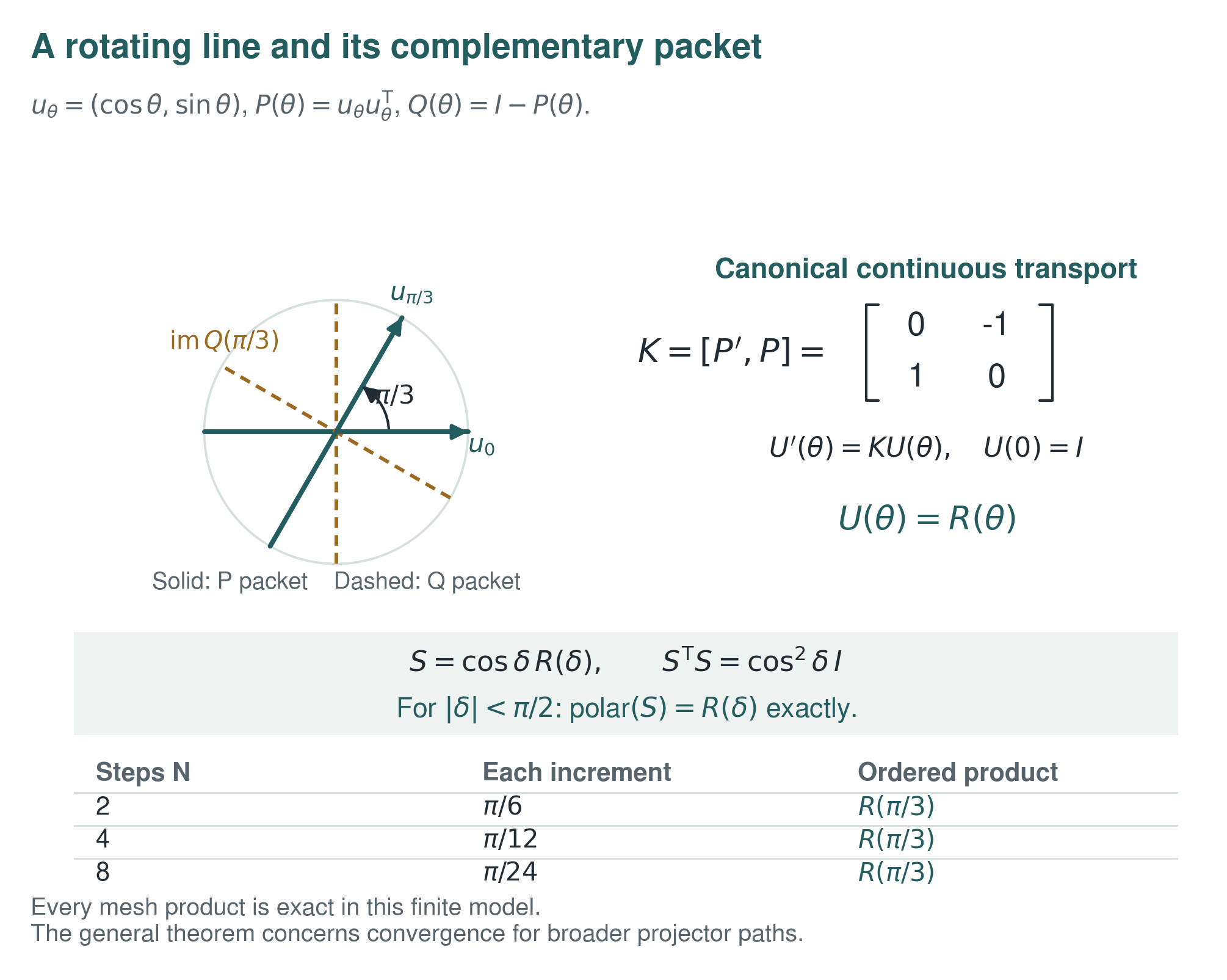
Each direct rotation maps a sampled packet exactly to the corresponding packet at the next sample. The product therefore preserves packet labels throughout the partition. Convergence compares this discrete product with the canonical continuous transport. The uniform estimate uses twice continuous differentiability in operator norm, as stated in the theorem.
Theorem 27.8: Convergence of sampled transports
Assume \(K\) is Lipschitz on \([0,T]\). For a partition
define
As the mesh \(|\pi|\) tends to zero,
in operator norm. There is a constant \(C\), depending only on \(T\), the supremum norm of \(K\), and its Lipschitz constant, such that
Read proof · Read statement and proof side by side · Permalink · Source line 1056 · Claim record · Lean coverage · Code · Worked examples
Proof of Theorem 27.8
On each interval, compare the exact propagator with the frozen exponential. Variation of constants and the Lipschitz bound give a local error bounded by a constant times the square of the interval length. Every factor is unitary, so multiplication does not amplify norms. Summing the local errors gives a bound by a constant times
Back to statement · Read statement and proof side by side · Permalink · Source line 1080 · Claim record · Lean coverage · Code · Worked examples
Corollary 27.9: Continuous holonomy from graph products
Assume the complete packet family is twice continuously differentiable in operator norm on \([0,T]\). If \(P_\alpha(0)=P_\alpha(T)\) for every \(\alpha\), then \(U(T)\) preserves every initial packet. Its restriction to each packet is the holonomy of the closed packet path. The products in Theorem 27.7 and Theorem 27.8 converge to these holonomies. The direct rotation product has the added property that every factor maps each sampled packet exactly to its successor.
Read proof · Read statement and proof side by side · Permalink · Source line 1090 · Claim record · Lean coverage · Code · Worked examples
Proof of Corollary 27.9
The transport identity in Theorem 27.2 gives packet preservation at the endpoint. The two convergence statements follow from Theorem 27.7 and Theorem 27.8.
Back to statement · Read statement and proof side by side · Permalink · Source line 1094 · Claim record · Lean coverage · Code · Worked examples
Example 27.10: A rotating line
In \(\mathbb R^2\), let
and let \(P(t)\) be the orthogonal projection onto the line spanned by \(v(t)\). The canonical transport is the ordinary rotation matrix
It carries the initial line and its orthogonal complement to the two moving packets. Products of short rotations converge to the same transport.
Standard fact 27.11: Curvature of a projected connection
Let \(P\) be a smooth orthogonal projector valued map on a parameter manifold. The connection
on the range bundle has curvature
Read proof · Read statement and proof side by side · Permalink · Source line 1115 · Claim record · Lean coverage · Code · Worked examples
Proof of Standard fact 27.11
For a section \(s\) satisfying \(Ps=s\),
Since \(ds=(dP)s+Pds\) and \(P(dP)P=0\), the surviving term is
Back to statement · Read statement and proof side by side · Permalink · Source line 1126 · Claim record · Lean coverage · Code · Worked examples
28 Realization data and limits of the calculus
On this page · Permalink · Source line 1137
The smooth transport theorem starts with a declared projector family. Applying it to a physical model requires a construction of that family and, where relevant, a separate continuum limit. Triviality of holonomy is a further geometric question. The curvature formula in Standard fact 27.11 is classical. Relating it to global holonomy requires geometric information as in [Kato1950], [Kato1995], [KobayashiNomizu1963].
An application begins by specifying the following objects:
an ambient nonlinear equation or continuation problem
the allowed correction space
a linear correction map or a correction complex
the defect whose class is to be tested
a packet decomposition or filtration compatible with the correction data
transition maps between refinement levels
transport maps when local solutions must be glued.
Once these objects are fixed, the cokernel and cone constructions are functorial by Theorem 21.3 and Theorem 21.11. Packet splitting and descent follow from Theorem 21.4, Proposition 21.6, and Corollary 21.12. Relative loss under coarsening is measured by Theorem 21.7.
Filtered lifting follows from Theorem 23.2, Theorem 23.6, and Theorem 23.8. Gluing and comparison of transport systems follow from Theorem 26.4 and Theorem 26.6. Smooth packet transport follows from Theorem 27.2 and Theorem 27.7.
Exact packet coordinates give a representation of the data. Solving the associated problem still requires the correction and lifting hypotheses. The correction map belongs to the problem data, and its cokernel is canonical relative to that choice. The cokernel may be infinite dimensional. In the Hilbert setting, the orthogonal obstruction projector requires closed range.
Coarse vanishing can erase a nonzero fine obstruction, and higher nonlinear terms can obstruct a problem whose linear class vanishes. A spectral sequence records which classes survive the later differentials. An application of finite graph holonomy or smooth projector transport to a continuum field theory requires the additional realization data just described.
Whenever a nonlinear continuation problem supplies a correction map, its residual can be recorded in an exact quotient or cohomology object. Under the stated hypotheses, these objects admit packet decomposition, filtered refinement, natural transport, and holonomy tests. They identify the obstruction that a correction or gluing step must address.