
2 Operations must survive their representations
On this page · Permalink · Source line 176
A representation is useful only to the extent that its intended operations remain meaningful.
On this page · Permalink · Source line 177
There are two different ways to change representation. An exact split representation retains the whole mathematical state in another space. A compression retains only part of it. The first can preserve arbitrary composition. The second needs additional conditions.
2.1 Exact packets and the hidden-return defect
On this page · Permalink · Source line 180
Let \(V,Z\) be vector spaces over a field. Let \(A:V\to Z\) be analysis and \(S:Z\to V\) synthesis, with \(SA=I_V\). Then \(AS\) is an idempotent on \(Z\). The map \(\mathcal E(T)=ATS\) represents a full-state operator \(T:V\to V\) on resolved coordinates. Direct multiplication gives
The resolved identity is \(AS\) on the compatible image \(A(V)\), not necessarily \(I_Z\) on arbitrary coordinates.
For a compression, reverse the splitting. Let \(C:V\to Z\) and \(R:Z\to V\) satisfy \(CR=I_Z\), and put \(P=RC\). The compressed operator is \(\Phi(T)=CTR\).
Proposition 2.1: Exact accounting of the discarded excursion
For any endomorphisms \(T,U\) of \(V\),
Thus compression preserves this composition precisely when the discarded excursion on the right vanishes. Full split encoding \(T\mapsto ATS\) preserves composition without that extra condition.
Read proof · Recorded Lean scope · Permalink · Source line 189
Proof
Expand the product \(\Phi(T)\Phi(U)=CTRCUR=CTPUR\) and subtract it from \(CTUR\). The identity for full split encoding follows from \(SA=I_V\) as computed above. These computations make no approximation and require no orthogonality.
Source relationship. Sufficient Resolution [SR], Theorems 2.1 and 2.3. The present proof reviews only these algebraic identities, not the complete forty-seven-page source or its full formal implementation.
Counterexample 2.2: A discarded coordinate returns
Take \(V=\mathbb R^2\), let \(C(x_1,x_2)=x_1\), let \(R(z)=(z,0)\), and let \(T(x_1,x_2)=(x_2,x_1)\). The compressed one-step map is zero. Yet \(T^2=I_V\), so \(\Phi(T^2)=I_Z\), while \(\Phi(T)^2=0\). The discarded second coordinate was not irrelevant to the two-step question.
This is the mathematical reason that a short successful readout is not enough. A representation may preserve what is visible now and lose a route by which hidden information becomes visible later. Packets identify the retained and residual components, but the decomposition alone does not prove the residual harmless.
2.2 A method can be transported without reconstructing everything
On this page · Permalink · Source line 207
Suppose source states \(z\in Z\) have operations \(F_a\), target states \(u\in U\) have operations \(G_{\tau(a)}\), and \(T:Z\to U\) is a translation. The operation-name map \(\tau\) is fixed. Let \(q\) and \(\bar q\) be matched readouts.
Theorem 2.3: Forward transport of a reusable method
If the source domain is invariant, and
then for every finite word \(w\),
Read proof · Recorded Lean scope · Permalink · Source line 210
Proof
The empty word gives \(TI_Z=I_UT\). Assume the first equality for a prefix. Invariance allows the next local equality to be applied on its successor, yielding \(TF_aF_w=G_{\tau(a)}TF_w=G_{\tau(a)}G_{\tau(w)}T\). Induction proves the first claim. Composition with the matched readout proves the second.
Source relationship. [MU], Theorem 6.1; the same local-to-continuation argument appears in OSL and Neuralese. No claim about a learned latent translator is imported. Boundary. The theorem is forward. It does not imply an inverse, matching of new target operations, cheap computation of \(T\), or that the source solver causally uses the represented state.
The sensor representation \((y,s)\) translates to \((b,s)\) through \(T(y,s)=(y\oplus s,s)\). Flipping the physical bit complements the first coordinate in either representation. The square commutes, and so does every repeated flip. The nuisance bit is never reconstructed because it has no role in this contract.
2.3 One quotient for several possible dynamics
On this page · Permalink · Source line 230
A stronger situation arises when the operator itself is uncertain. Let \(V\) be finite dimensional, let \(T_a^\theta\) be finitely many candidate linear operators, and let \(A_a\) be one complete candidate system chosen as reference. A model index \(\theta\) is fixed during the initial comparison. Let \(Q:V\to Y\) be the same linear readout for every candidate.
Define \(D_a^\theta=T_a^\theta-A_a\) and the propagated discrepancy space
It can be constructed by starting with the sum of the discrepancy ranges and repeatedly adding their images under the reference actions. In finite dimension this increasing sequence stops. Immediate invisibility \(QD_a^\theta=0\) alone does not guarantee \(QE=0\).
Theorem 2.4: A common observable quotient
The following conditions are equivalent:
\(QT_w^\theta=QA_w\) on all of \(V\), for every fixed candidate \(\theta\) and every word \(w\).
\(E\subseteq\ker Q\).
There is a surjective linear \(r:V\to Z\), common updates \(G_a\), and a readout \(\bar Q\) with \(rT_a^\theta=G_ar\) and \(Q=\bar Qr\) for every \(a,\theta\).
Under these conditions, \(V/E\) is a common quotient and also predicts the output when the candidate index changes between operations.
Read proof · Recorded Lean scope · Permalink · Source line 239
Proof
Assume the first condition. For every \(a,\theta,w\), equality as operators on all of \(V\) gives
The last equality applies the premise to the word executing \(a\) and then \(w\). Spanning proves \(E\subseteq\ker Q\).
Conversely, \(E\) is invariant under every \(A_a\) by construction, and contains the entire range of each difference \(D_a^\theta\). Hence \(T_a^\theta E\subseteq E\), and every candidate induces the same map \(G_a([v])=[A_av]\) on \(V/E\). Since \(QE=0\), the readout descends. This proves the third condition. Composing its equalities yields the first condition. The same induction permits a different \(\theta\) at each step because the quotient map and update remain shared.
Source relationship. [GA], Theorem 13.1, “Exact common quotient for structured model uncertainty.” The all-initial-vectors hypothesis is retained.
For example, let \(Q(x_1,x_2,x_3)=x_1\) and let every candidate act as
Then \(E\) is contained in the third coordinate and remains invisible. The two-coordinate method \((x_1,x_2)\mapsto(x_1+x_2,x_2)\) is exact, although the hidden dynamics are not identified.
The conclusion would be different if a later action moved the third coordinate into the first. That change enlarges \(E\) beyond \(\ker Q\). It invalidates the use of this quotient, not the theorem that justified the former one.
2.4 An algebraic packet is not automatically a probability
On this page · Permalink · Source line 268
The previous sections concern linear representations. Bayesian correction will require more: a nonnegative state with a well-defined total mass. Those requirements belong to a declared domain, not to the spelling of its coordinates.
Let \(\mathcal K\) be a convex cone in a real vector space, and let \(\lambda\) be linear and strictly positive on every nonzero member of \(\mathcal K\). Its normalized states satisfy \(v\in\mathcal K\) and \(\lambda v=1\). A coordinate change can send \(\mathcal K\) to a cone containing negative coordinates without changing those states' probability meaning. Conversely, an arbitrary signed component of a valid state need not itself be valid.
Proposition 2.5: When complete packets are genuine probability components
Let \(P_1,\ldots,P_m\) be linear maps with \(\sum_iP_i=I\). If every \(P_i\) preserves \(\mathcal K\), each normalized \(v\in\mathcal K\) has the mixture decomposition
Every zero-weight component is zero. If \(\mathcal K=\mathbb R^d_{\ge0}\) and the \(P_i\) are also idempotent, they must be disjoint diagonal coordinate selections. Orthogonal completeness alone does not imply a probability mixture.
Read proof · Recorded Lean scope · Permalink · Source line 273
Proof
Cone preservation places \(P_iv\) in \(\mathcal K\), so its mass is nonnegative. Strict positivity says that a member of this cone with zero mass is zero. Applying \(\lambda\) to the complete decomposition gives \(\sum_iw_i=\lambda v=1\). Dividing every nonzero component by its mass proves the mixture identity.
On the nonnegative coordinate cone, preservation is equivalent to nonnegative matrix entries, as is seen by applying a matrix to every standard basis vector. Because the matrices sum to \(I\), their nonnegative off-diagonal entries must all vanish. An idempotent diagonal entry satisfies \(x^2=x\), hence is zero or one. The diagonal sums are one, so each coordinate is selected by exactly one map. Finally, completeness and orthogonality without positivity do not give the first premise, as the following example shows.
Source relationship. Large Signal Model Foundations [LSM], Proposition 30, physical page 40. Only this finite packet argument and the joint-closure result below are admitted from that source at this stage.
Counterexample 2.6: An exact detail component has negative probability mass
For \(p=(3/4,1/4)^\top\), the orthogonal average and detail projectors are
They sum to the identity and produce \((1/2,1/2)^\top\) and \((1/4,-1/4)^\top\). The components reconstruct \(p\) exactly, but the detail has zero total mass without being zero. Normalizing it as a belief is undefined. Clipping its negative entry and normalizing the resulting sum would instead produce \((3/5,2/5)^\top\), a different belief.
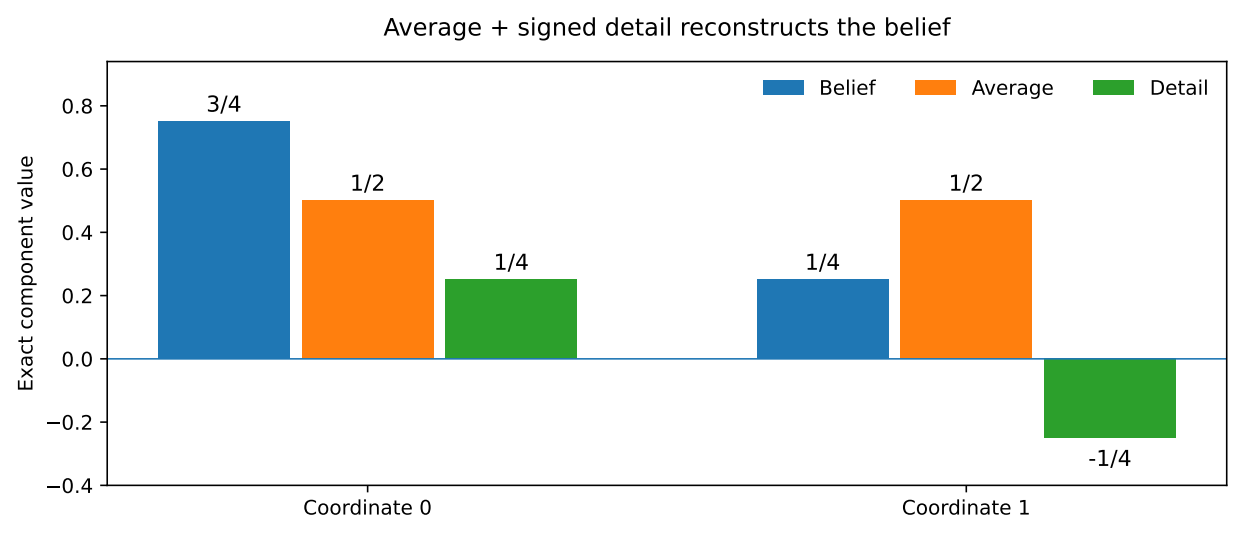
This distinction supplies the interface to the next chapter. A signal packet may describe a discrepancy, a coordinate, or a component of an operator. A belief represents nonnegative mass over alternatives. Moving between them requires a domain-preserving map. No learned signal architecture is inferred from this algebraic admission.
What is now available
On this page · Permalink · Source line 304
We have a declared method that preserves the selected outputs. But a predictive quotient need not retain the relationships needed for new evidence. The next chapter changes the retained object from a current physical coordinate to a set or distribution of candidate worlds.