
1 From evidence to a reusable state
On this page · Permalink · Source line 100
The first question is not how much state to store. It is which distinctions are accessible.
On this page · Permalink · Source line 101
Let \(\Omega\) be a finite nonempty set of possible worlds. A world may include a physical state, a fixed model index, and an origin tag. An observation record is a function \(r:\Omega\to H\). A target is a function \(t:\Omega\to Y\). All codomains used below are nonempty. We work on attained records \(r(\Omega)\), so no arbitrary interpretation of an impossible record is needed.
Proposition 1.1: A record determines a target exactly on its fibres
There exists \(d:r(\Omega)\to Y\) with \(d(r(\omega))=t(\omega)\) for every world if and only if
Read proof · Recorded Lean scope · Permalink · Source line 104
Proof
Necessity follows because a function assigns one value to one input. For sufficiency, define \(d(h)\) to be \(t(\omega)\) for any world with \(r(\omega)=h\). Such a world exists for attained \(h\), and the hypothesis makes the choice immaterial. The resulting decoder satisfies the required equation.
Source relationship. Grounded Abstraction [GA], Proposition 3.2 and Theorem 3.4; Machine Understanding [MU], the representation and sender-access criteria. This is the shared elementary factorization argument, stated once.
The proposition is an information statement, not a runtime bound. The table defining \(d\) could be large. Nor does the mere existence of \(d\) teach a learner how to find it. A proof that a suitable decoder exists and a justified account of its acquisition remain separate.
1.1 The sensor used throughout the book
On this page · Permalink · Source line 117
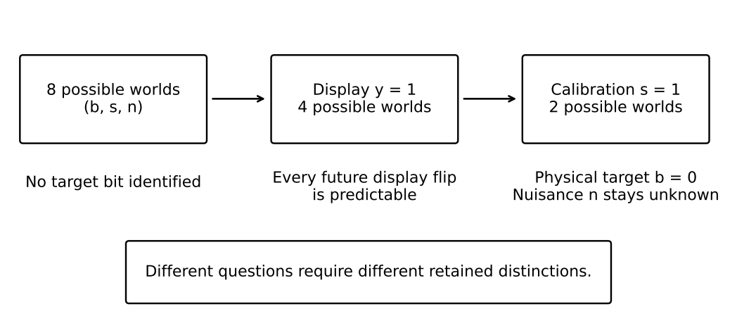
Write a world as
The physical target bit is \(b\). The sensor convention is \(s\). The nuisance bit \(n\) never affects the operations or outputs of the initial contract. The display is
where \(\oplus\) is addition modulo two. A permitted control \(f\) flips the physical bit and leaves \(s,n\) unchanged. Consequently the next display is \(1-y\).
An agent given only \(y\) can predict every future display under repeated flips: after \(k\) flips it is \(y\oplus(k\bmod2)\). It cannot determine the current physical bit. Worlds \((0,0,0)\) and \((1,1,0)\) share display zero and have different targets. The obstruction is the fibre of the available record, not a shortage of computational effort.
Calibration is a separate, nondestructive observation \(c(\omega)=s\). When calibration is permitted and trustworthy, the joint record \((y,s)\) determines \(b=y\oplus s\). Adding a blank field called “sensor convention” does not provide this information. The observation operation, its interpretation, and its cost must be part of the contract.
| Available record | Number of values | Determines display? | Determines physical bit? |
|---|---|---|---|
| \(y\) | 2 | Yes | No |
| \((y,s)\) | 4 | Yes | Yes |
| \((b,s,n)\) | 8 | Yes | Yes, with unused detail |
1.2 One answer versus every permitted continuation
On this page · Permalink · Source line 143
Let \(X\) be a finite nonempty state space. Let \(\mathcal A\) be a finite alphabet of total deterministic operations \(F_a:X\to X\), and let \(q:X\to Y\) be the protected output. A word \(w=a_1\cdots a_k\) executes \(a_1\) first. Thus \(F_w=F_{a_k}\cdots F_{a_1}\), and the empty word denotes the identity.
Define behavioral equivalence by
The empty word protects the present output. The other words protect its permitted future uses.
Theorem 1.2: Evidence-initialized behavioral state
A finite predictor initialized only from \(r(x)\), updated only by the operation names, and exact for all protected continuation outputs exists if and only if
When it exists, \(X/{\sim}\) supplies a predictor with the smallest possible number of initialized states. Its updates are \(\bar F_a([x])=[F_ax]\) and its readout is \(\bar q([x])=q(x)\).
Read proof · Recorded Lean scope · Permalink · Source line 152
Proof
If two initial records are equal, a deterministic predictor has the same initialized state. Applying the same subsequent operations produces the same predicted outputs. Exactness therefore requires behavioral equivalence.
For the converse, equivalent states have equivalent successors: an output after \(F_a\) followed by \(w\) is one of the outputs in the defining family. Hence \(\bar F_a\) is well defined. The empty word makes \(\bar q\) well defined. The fibre premise gives a well-defined initializer \(d(r(x))=[x]\). Induction on word length proves exactness. Finally, behaviorally distinct states cannot initialize the same predictor state, since some continuation separates their outputs. Every exact predictor therefore needs at least one initialized value for each class, and the quotient attains that number.
Source relationship. [GA], Theorem 3.4, and [MU], Theorem 4.1. The two source versions are consolidated, not counted as independent discoveries.
In the sensor, the display task has two behavioral states. Changing the protected output to \((y,b)\) yields four behavioral states. The old record still has only two values and cannot initialize the enlarged quotient. The new task has exposed a real information requirement.
1.3 Why a statistical law is not an observed record
On this page · Permalink · Source line 168
A parameter can determine a distinct probability law while every finite sample remains possible under several parameters. For instance, Bernoulli parameters \(1/3\) and \(2/3\) assign positive probability to every finite binary string. No estimator based on one such string can be certainly correct for both parameters. The laws differ, but their finite supports overlap.
A correct uncertainty record can be the appropriate output in this setting. Calling the most probable world “identified” would silently replace an error-free claim with a probabilistic one. Chapter 3 gives the corresponding probability update explicitly.
What is now available
On this page · Permalink · Source line 173
We have a criterion for an initialized predictive state, but no automatic guarantee that an arbitrary coordinate manipulation preserves it. The next chapter studies operations on a representation. Its input is a declared state map and operation family, not an assumed learned encoder.