
3 Memory that remains open to correction
On this page · Permalink · Source line 307
A useful memory preserves the distinctions by which its own conclusions can be revised.
On this page · Permalink · Source line 308
Let \(t:\Omega\to Y\) be the current target. A candidate set \(V\subseteq\Omega\) records worlds still possible. The empty set is allowed and means that the represented candidates contradict the admitted evidence. It is not a successful identification.
Let \(\mathcal E\subseteq{\mathcal P}(\Omega)\) contain \(\Omega\) and be closed under intersection. In this chapter the world does not change when an evidence event is received. The update is \(V\mapsto V\cap E\). Physical actions and their effects will return in Chapter 5.
3.1 A state sufficient for every later filter
On this page · Permalink · Source line 313
Define the correction signature
It records what each admitted future filter would leave of the possible target values.
Theorem 3.1: Minimal exact memory for a correction contract
Equality of \(\Sigma\) is a congruence for every update \(V\mapsto V\cap E_0\). The signature supports the current target set and its exact update after every finite evidence sequence. Any deterministic retained state supporting the same readouts and updates on all candidate subsets must distinguish every two distinct signatures. Thus the image of \(\Sigma\) has the least possible cardinality for this contract.
Read proof · Recorded Lean scope · Permalink · Source line 320
Proof
If \(\Sigma(V)=\Sigma(W)\), then for each \(E\),
Intersection closure supplies the coordinate \(E_0\cap E\), so the updated signatures agree. The \(\Omega\) coordinate is the present target set. Induction gives every finite sequence.
If signatures differ, one admitted event produces distinct target sets. A memory that merged those candidates would update identically and return the same answer on that event, contradicting exactness. Hence each signature needs its own state. The signature construction attains the lower bound.
Source relationship. [GA], Theorem 5.2. This is a behavioral quotient of the correction process, not a claim that all candidate sets must be stored literally.
3.2 An exact count for partition evidence
On this page · Permalink · Source line 334
Suppose \(C_1,\ldots,C_m\) partition \(\Omega\) into nonempty cells and the admitted events are exactly their unions. Let
The occupancy memory retains whether a candidate exists in each attainable cell–target pair.
Corollary 3.2: The size of partition correction memory
On all subsets of \(\Omega\), correction signatures are exactly distinguished by these occupancy records. There are \(2^r\) signatures, and \(r\) fixed binary bits are necessary and sufficient to encode them.
Read proof · Recorded Lean scope · Permalink · Source line 341
Proof
An individual-cell filter reveals the target values occupied in that cell, so the signature determines occupancy. Conversely, occupancy determines the target values left by any union of cells. Every subset of \(D_t\) occurs: select one world from each included nonempty cell–target intersection and none from excluded intersections. Those intersections are disjoint. Thus there are precisely \(2^r\) possible records. The preceding theorem and binary counting give necessity, while the occupancy vector supplies sufficiency.
Source relationship. [GA], Corollary 5.3. The word “exactly” in the evidence premise is essential.
For the sensor, the four cells are fixed pairs \((b,s)\) with either nuisance value. Calibration and display evidence generate their unions. The target is \(b\), so there are four attainable cell–target pairs. Candidate membership uses eight bits for eight worlds. Correction memory uses four bits for sixteen possible occupancies. The current target set alone has four possibilities and needs only two bits, but is not sufficient for later calibration.
For example,
have the same possible target set \(\{0,1\}\). After the event \(s=0\), one leaves target zero and the other target one. Their different associations are operationally relevant.
Counterexample 3.3: A new evidence event changes the required memory
Take one cell \(\Omega=\{u,v\}\) and a constant target. The singleton candidate sets have the same old occupancy. If the event \(\{u\}\) is added, filtering one singleton gives a target value while filtering the other gives contradiction. A record sufficient for the old event algebra is insufficient for the larger one.
3.3 Noisy correction is not elimination
On this page · Permalink · Source line 361
A likelihood can be small without being zero. Deleting a candidate because an observation was surprising can invalidate a correct noise model. We therefore specify a separate probability contract.
Let \(M\in\mathcal M\) be a fixed model with prior \(p(m)\). Let an experiment have likelihood \(L_m(o)\) on a finite nonempty observation alphabet \(\mathcal O\). A reporting channel \(B(o,z)\), independent of the model conditional on \(o\), creates a retained report \(Z\). The joint law is
Posterior distributions are defined only on positive-probability events.
Theorem 3.4: When a report preserves every Bayesian correction
The following are equivalent:
For every prior, the posterior after \(o\) equals that after \(z\) on every positive-probability pair \((o,z)\).
The equality holds for one prior positive on every model.
There is a stochastic kernel \(\rho(o\mid z)\) such that
\[ L_m(o)B(o,z)=Q_m(z)\rho(o\mid z)\quad\text{for all }m,o,z. \]
The reconstruction in the last condition refers to the actual joint experiment, not an unrelated simulation with matching marginals.
Read proof · Recorded Lean scope · Permalink · Source line 370
Proof
The first condition implies the second. Under a positive prior, define \(\rho(o\mid z)=\Pr(o\mid z)\) whenever \(z\) has positive probability. For a positive pair, posterior equality yields
Substituting Bayes' formula and cancelling positive \(p(m)\) gives the factorization. A zero-probability pair under a positive prior has \(L_m(o)B(o,z)=0\) for all \(m\); its conditional weight is zero. If \(z\) is impossible for every model, assign any probability row to \(\rho(\cdot\mid z)\) because both sides vanish.
Conversely, the factorization makes the likelihood of \((o,z)\) a model-independent multiple of the likelihood of \(z\). Normalization under any prior therefore gives \(p(m\mid o,z)=p(m\mid z)\). Since the common channel only reads \(o\), the same positive-pair posterior equals \(p(m\mid o)\). This proves the first condition.
Source relationship. [MU], Theorem 12.1. The full-support and zero-probability cases are included in the proof.
The theorem permits removal of an independent nuisance flag. It does not permit removal of every association. Consider two priors on \((b,s)\), with rows indexed by \(b\) and columns by \(s\):
Both individual marginals are uniform. A noisy calibration reports \(s\) correctly with probability \(3/4\), independently conditional on the fixed world. The probability of report one is \(1/2\) under both priors. After that report, however, the target posteriors are \(3/4\) and \(1/4\). Separate target and sensor marginals cannot support this correction. Their association matters even though neither marginal changed.
These examples do not identify a universally optimal memory. They identify the least information required by a specified correction contract. A new likelihood, a newly admitted model, or a different target can change that requirement.
3.4 A record must close under prediction as well as correction
On this page · Permalink · Source line 404
The static Bayesian theorem preserves one update of a fixed candidate model. A continuing reasoner also predicts what happens between observations. The same compressed record must support both operations. Otherwise a valid posterior can become an inadequate input to the very next prediction.
First consider a known finite state set \(X\) with row-stochastic transition matrices \(K_a(x,x')\). We retain column-vector probability distributions. A partition \(\pi\) has aggregation \(C_\pi(z,x)=1_{\{\pi(x)=z\}}\), so prediction is \(p\mapsto K_a^\top p\). For each permitted observation symbol \(o\), let \(\ell_o(x)>0\) be its specified likelihood. When these are a complete report alphabet, assume also \(\sum_o\ell_o(x)=1\).
A mandatory partition \(\pi_0\) with at least two blocks protects the target distinctions. We seek a refinement that supports every prediction and each separate Bayesian update for every prior. The observation is an operation available in its own right. This is stronger than inspecting only a chosen combined transition-and-report schedule.
Theorem 3.5: Least refinement closed under prediction and correction
First split \(\pi_0\) by the complete vectors \((\ell_o(x))_o\), obtaining \(\pi_{\rm init}\). Then repeatedly split current blocks by
where \(B\) runs over the current blocks. The process stops after at most \(|X|-|\pi_{\rm init}|\) strict refinement rounds. Its final partition is the unique coarsest refinement of \(\pi_0\) for which all specified predictions admit stochastic coarse transitions and all separate Bayesian updates admit fixed strictly positive coarse likelihoods for every prior.
Read proof · Recorded Lean scope · Permalink · Source line 411
Proof
At a stable partition the probability of reaching each coarse block depends only on the current block. These sums define a stochastic coarse transition and yield \(C_\pi K_a^\top=\bar K_a^\top C_\pi\), first on point masses and then by linearity. Likelihoods are constant within final blocks. Grouping the numerator and normalizer by those blocks therefore commutes with every Bayesian update.
For minimality, take any admissible refinement \(\eta\) of \(\pi_0\). It has at least two blocks. Fix a strictly positive fine likelihood \(\ell\) and a strictly positive coarse likelihood \(\bar\ell\) inducing its assumed update. For states \(x,y\) in one block and \(z\) in a different block, compare priors assigning half their mass to \(x,z\) and to \(y,z\). Their coarse priors agree. Equality of the posterior odds gives
Thus \(\ell(x)=\ell(y)\), and \(\eta\) refines the first likelihood split. Coarse likelihoods may differ by a positive scale for each observation without changing this conclusion.
If \(\eta\) refines a current partition, each current block is a union of \(\eta\) blocks. Exact prediction under \(\eta\) makes the probability of reaching each such union constant inside every \(\eta\) block. Hence \(\eta\) refines the next split too. Induction proves that every admissible refinement refines the terminal one. Each strict round increases the block count, proving the bound. Coarseness determines the partition uniquely, up to naming its blocks.
Source relationship. [LSM], Proposition 9 and Proposition 12, physical pages 11–14; Bayesian necessity also appears in PRIQ [PRIQ], Theorem 5.6. The proof includes the two-block and strict-positivity premises rather than importing them by a cross-reference.
For the sensor, the mandatory display partition has two blocks. A noisy calibration that reports \(s\) correctly with probability \(3/4\) splits it into the four \((b,s)\) blocks. The nuisance bit remains merged. The physical flip maps these four blocks among themselves, so the transition stage introduces no further split. The representation is now closed for both prediction and correction, not merely for today's display.
Refinement can also propagate backward through dynamics. In a separate four-state example, the mandatory partition is \(\{0,1,2\}\mid\{3\}\) and the deterministic successors are \((0,2,3,3)\). A constant likelihood adds no information. Transition signatures first isolate state 2, then separate 0 from 1. The final partition is discrete. The reason for the second split is a future observable difference, not a newly sampled measurement.
The construction uses complete tables. It does not acquire those tables, certify their physical accuracy, or guarantee a finite encoding of every posterior coordinate. Its least-state statement concerns the specified separate operations and all priors. Different admissible schedules or reachable-prior restrictions can justify another quotient.
3.5 Retain the joint law of the report and the next state
On this page · Permalink · Source line 437
A general experiment can change the state and report correlated information about the change. Describing its transition and report marginals separately is then insufficient. Let
be a nonnegative finite instrument with \(\sum_{o,x'}K_{a,o}(x',x)=1\) for every \(a,x\). This notation is column-oriented: \(K_{a,o}p\) is an unnormalized post-experiment distribution. It specifies an experiment's physical change and its observation in one object.
For a surjection \(\pi:X\to Z\), let \(C\) sum probabilities over its fibres. Write
when the denominator is positive. Zero mass means an impossible report under that prior, not an arbitrarily assigned posterior.
Theorem 3.6: One quotient for reports, posteriors, and feedback
A nonnegative normalized coarse instrument \(\bar K_{a,o}\) satisfies
if and only if, for all \(a,o,z'\),
is constant as \(x\) varies within any one input fibre. Such a coarse instrument is unique. Equivalently, it preserves for every prior both the report probabilities and the aggregated positive-probability posteriors:
Starting from \(Cp_0\), these identities preserve every finite joint action/report law and every corresponding coarse posterior under one common policy that uses only the previously observed action/report history. This includes randomized policies with the same history-conditional action probabilities.
Read proof · Recorded Lean scope · Permalink · Source line 451
Proof
Applying the matrix identity to a point mass proves necessity of the fibre condition. Conversely, use the common sums to define each column of \(\bar K_{a,o}\). They are nonnegative. Summing across \(z',o\) partitions the fine successor set and gives column mass one. The definition proves the matrix equality on point masses, hence on every vector. Surjectivity gives uniqueness.
Because \(\mathbf1_Z^\top C=\mathbf1_X^\top\), the matrix equality gives equal report masses. Dividing it by a common positive mass gives equal aggregated posteriors. Conversely, equality of masses and positive-mass posteriors gives the unnormalized matrix equality on every prior. If the common mass is zero, both unnormalized vectors are zero by nonnegativity. Point masses finish that direction.
For a history \(h\), keep unnormalized states \(u_h,\bar u_h\). Initially \(\bar u_\varnothing=Cu_\varnothing\). After choosing action \(a\) with common probability \(\gamma(a\mid h)\) and receiving \(o\), the next states are \(\gamma(a\mid h)K_{a,o}u_h\) and \(\gamma(a\mid h)\bar K_{a,o}\bar u_h\). The intertwining identity preserves their aggregation. Induction gives equal mass for every history, including zero-mass histories. Normalization on positive histories gives the posterior statement. Stopping decisions based on the same history can be included as matching terminal choices.
Source relationship. Selected synthesis of the positive-transfer and filtering arguments in [PRIQ], Theorems 5.2, 6.1 and 6.3, and the projected-law construction in AVOC [AVOC], Theorem 4.5. The joint instrument and feedback formulation is proved here. No entire nonlinear source theorem or Lean implementation is imported.
Counterexample 3.7: Correct marginals with an incorrect correction
Two fine current states have the same retained label. From the first, the next retained state and report are \((0,0)\) or \((1,1)\), each with probability \(1/2\). From the second they are \((0,1)\) or \((1,0)\), again equally likely. In both cases the next-state marginal is uniform and the report marginal is uniform. After report one, however, the next retained state is certainly one in the first case and certainly zero in the second. No common filter based only on the old label can realize both. The joint fibre condition detects exactly the lost association.
Preserving only normalized posteriors is weaker still. A report coin independent of the hidden state leaves every prior unchanged whether its success probability is \(1/4\) or \(3/4\). Those two instruments have identical posterior maps but different report laws. A planner that prices later branches needs those probabilities. In the exact instrument theorem the evidence scale is fixed, rather than silently discarded during normalization.
3.6 Small law error and a rare conditional history
On this page · Permalink · Source line 481
Approximate models must be compared before declaring their posteriors close. Let \(\widetilde K\) be a normalized instrument on the same coarse state and report alphabets. Suppose, at step \(t\), every relevant action and fine state satisfy
This is a bound on a complete report/next-state distribution, not on an isolated matrix entry. Assume \({d_{\mathrm{TV}}}(Cp_0,\widetilde p_0)\le\delta_0\) with nonnegative \(\delta_0,\epsilon_t\). Both models run the same history-based policy. Coarse states recorded in the comparison below are analytical coordinates, not extra observations supplied to that policy.
Proposition 3.8: A whole-history bound with an explicit conditioning cost
At horizon \(H\), the distributions \(P_H,\widetilde P_H\) of the full coarse-state and action/report histories satisfy
The same bound holds after forgetting any of those history coordinates. For an observed history event \(E\) with probabilities \(p_E,\widetilde p_E>0\), the conditional final coarse-state distributions obey
If either event probability exceeds \(d_H\), the other is necessarily positive.
Read proof · Recorded Lean scope · Permalink · Source line 489
Proof
Condition on a complete coarse history with positive fine probability. Its hidden current-state distribution is a mixture of states in the last coarse fibre. Convexity of total variation makes the true next report/coarse-state row differ from the declared row by at most \(\epsilon_t\). Mixing over a common action kernel preserves this bound. Extend the two old history laws first through the same declared row. Total variation cannot increase under a common stochastic kernel, by the triangle inequality and row sums. Replacing those rows with the true conditional rows adds at most \(\epsilon_t\), weighted by a total history mass of one. Hence the history distance at the next step is at most the old distance plus \(\epsilon_t\). Induction and the cap one prove the first claim. Summing over forgotten coordinates is also a stochastic map, proving the second.
For conditioning, let \(u,v\) be the restrictions of the two history laws to \(E\), with masses \(p_E,\widetilde p_E\). The difference on the complement has \(\ell^1\) norm at least \(|p_E-\widetilde p_E|\). Thus
Adding and subtracting \(v/p_E\) bounds the conditional distance by \(d_H/p_E\). Interchanging the laws gives \(d_H/\widetilde p_E\), so the smaller of these bounds has the displayed maximum denominator. Projection to the final state cannot increase the distance. Finally, the probability of any event changes by at most total variation, which proves positivity when one mass exceeds \(d_H\).
Source relationship. Finite probability-instrument specialization of [LSM], Propositions 43–44, with the joint retained-state record made explicit. The symmetric conditioning form follows by applying the same elementary bound in both directions. [PRIQ], Section 9 supplies the complementary stepwise posterior-error perspective.
Counterexample 3.9: A rare report carries the entire discrepancy
Two joint laws place mass \(1-\delta\) on the same ordinary outcome. On a report event \(E\) of mass \(\delta>0\), one puts all mass on retained state zero and the other on retained state one. Their whole-law distance is \(\delta\), while their conditional distance after \(E\) is one. The factor involving event probability is therefore essential. This is a finite-law statement, not an empirical estimate of a sensor error.
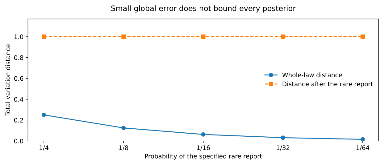
The bound compares one policy across two models, not independently optimized controllers. Chapter 5 supplies the uniform comparison needed for re-optimization. First, the next chapter asks what decisions and explanations the corrected record can justify.