
5 One investigation, one resource budget
On this page · Permalink · Source line 591
A possible answer, an affordable observation, and a small program must belong to the same workflow.
On this page · Permalink · Source line 592
Let \(X\) be a finite nonempty state space. It includes every origin tag, permission, background record, and history variable that affects the stated behavior. An experiment \(e\) is allowed on a domain \(D_e\subseteq X\), has a deterministic successor \(f_e:D_e\to X\), a report \(o_e:D_e\to O_e\), and a fixed nonnegative integer resource vector \(c_e\).
A current support \(V\ne\varnothing\) records possible states. The experiment is permitted only if \(V\subseteq D_e\). After report \(o\), the possible post-experiment states are
Only nonempty report branches are retained. If the target concerns a past value, that value must survive as an immutable tag. Resetting the current state is not recovering its history.
A terminal artifact \(a\) is acceptable only if every fixed recipient succeeds in every state of \(V\). Its worst-case terminal cost is \(g_a(V)\), computed componentwise. A controller is a literal finite tree with one record per experiment or terminal node. Stored memory counts all branches, including those not visited in one execution.
5.1 The complete finite frontier
On this page · Permalink · Source line 603
Let \(\mathcal P_h(V)\) be the nondominated pairs \((v,m)\) of worst-case online resource vectors and stored-record counts attainable by successful trees with at most \(h\) experiment steps. At depth zero the available pairs are
At greater depth retain those stops and, for each uniformly permitted experiment and one feasible child pair \((v_o,m_o)\) for every nonempty branch, form
A profile dominates another when it is no larger in every resource coordinate and strictly smaller in at least one. The maximum is componentwise. An impossible child contributes no tree; it is not a zero-cost branch.
Theorem 5.1: Exact joint feasibility for explicit controllers
This recurrence gives exactly the nondominated resource profiles of successful depth-bounded controllers. Every retained pair has a concrete tree witness. A common online and storage budget is feasible if and only if it bounds one retained pair. Removing dominated child profiles does not change feasibility under any componentwise budget.
Read proof · Recorded Lean scope · Permalink · Source line 614
Proof
At zero depth the only possibilities are acceptable terminals, whose profiles are exactly the stated stops. At positive depth a successful tree either stops or begins with one uniformly allowed experiment. Every possible report needs a successful child on precisely \(V_{e,o}\). By induction those children have profiles in the lower-depth attainable set. Worst-case online cost is the root cost plus their componentwise maximum. Complete tree storage is one plus the sum of all child records.
Conversely, combining any allowed root with a successful child for every report constructs a successful tree with that profile. This proves exact enumeration before pruning. Replacing a dominated child by a dominating one cannot increase either a coordinatewise maximum or a sum of record counts, and does not change its supported initial set. Thus Pareto pruning preserves every feasible budget and every retained profile has a witness.
Source relationship. [MU], “A joint resource certificate for fixed recipients,” and [SII], Theorem 6.2. The scalar-cost repair case is a specialization, not a different composition theorem.
The recurrence can be expensive. It is a finite mathematical characterization, not an efficient general learner. It assumes its transition and acceptance tables. Their discovery and checking are preparation costs, not free consequences of the existence theorem.
Counterexample 5.2: Two separate optima do not form one controller
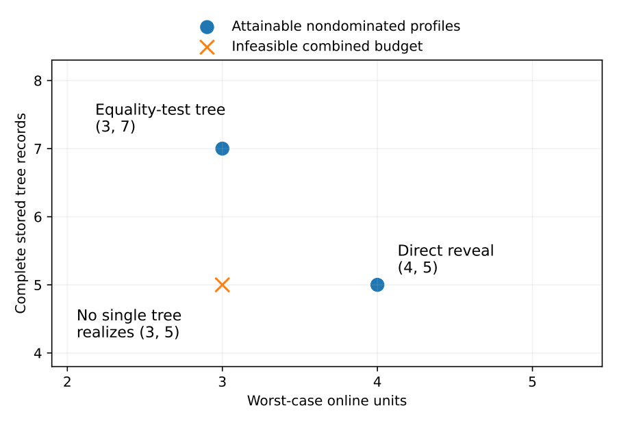
There are four immutable cases, each requiring its own terminal answer. A direct observation of the case costs four units and gives a five-record tree including four terminals. Unit-cost equality tests can identify the case in at most three tests with seven records. Terminal answers have zero online cost in this particular example. The frontier is \((4,5)\) and \((3,7)\). The mixed budget \((3,5)\) is infeasible: an all-equality successful tree needs four leaves and at least seven records; any tree using the direct observation on a reachable path costs at least four.
5.2 When a checked candidate can end the search
On this page · Permalink · Source line 635
Consider \(n\ge1\) immutable cases with total nondestructive binary unit-cost queries. Every unit-cost repair succeeds in exactly one case, and every case has a repair. A controller must succeed certainly in every case.
Theorem 5.3: A candidate attaining both lower bounds is optimal
Every successful controller has worst-case work at least \(1+\lceil\log_2n\rceil\) and literal storage at least \(2n-1\). A checked controller attaining both bounds and the requested horizon realizes the entire nondominated work/storage frontier.
Read proof · Recorded Lean scope · Permalink · Source line 638
Proof
Distinct cases cannot end at the same successful repair leaf, so at least \(n\) leaves are reachable. A binary tree of query depth \(d\) has at most \(2^d\) leaves, giving \(d\ge\lceil\log_2n\rceil\). The terminal repair adds one unit.
Let \(l\) be the number of leaves and \(i_1,i_2\) the counts of unary and binary internal nodes. Counting tree edges gives \(i_1+2i_2=i_1+i_2+l-1\), hence \(i_2=l-1\). Total records are \(2l-1+i_1\ge2n-1\). A successful candidate at both coordinatewise lower bounds dominates every other attainable cost profile. Its validity and horizon check make it an actual member of the frontier, leaving that pair as the whole nondominated frontier.
Source relationship. [SII], Theorem 11.1. The assumptions exclude destructive resets and repairs that succeed on several cases.
For eight possible defective cells, equality-first diagnosis requires seven queries in the worst case, while three coordinate-bit queries identify the cell. Including repair gives costs eight and four, respectively. Both literal trees have fifteen records. Faster execution has not eliminated the cost of storing the procedure.
This eight-cell example is separate from the eight-world sensor. The sensor has only four action-relevant \((b,s)\) pairs and an irrelevant nuisance coordinate. Confusing hidden-world cardinality with the number of required repair distinctions would import a false lower bound.
5.3 Expected-cost inquiry uses the report probabilities
On this page · Permalink · Source line 653
The preceding frontier certifies worst-case execution and complete tree storage for deterministic observations. A noisy report requires a different optimization. Expected cost weights each future branch by its probability. A low expectation is not a hard execution budget, and neither replaces the cost of storing the whole controller.
Use the finite instrument of Theorem 3.6, with fine belief \(p\) and coarse belief \(q=Cp\). At \(q\), a finite set of experiments \(A(q)\) is permitted, and a nonempty finite set of terminal decisions \(D(q)\) is available. These catalogues must be identical for every fine belief with the same \(q\). Stopping with decision \(d\) has loss \(\ell_d(\pi(x))\) in fine state \(x\), so its conditional risk is \(\langle q,\ell_d\rangle\). An experiment has a finite nonnegative charge \(c_a(q)\), identical on the fine and coarse side. All history variables affecting permissions, charges, or targets must be included in the declared state.
Let \(J_h(p)\) be the least expected charge plus terminal loss attainable using at most \(h\) further experiments, with terminal decisions permitted at any step. It is defined by finite observation trees, not by a hidden-state controller. Its coarse recurrence is
An empty experiment catalogue leaves only stopping. Impossible reports do not receive invented posteriors.
Theorem 5.4: The same compressed belief supports the same inquiry
Under the exact instrument quotient and the common loss, charge, and catalogue assumptions above,
Every first-action value and optimal first-action set agrees. A minimizing coarse-belief policy produces a fine-model optimal history-based policy, including its stopping decision. Finite minimizing trees exist. The result supplies neither an efficient synthesis algorithm nor a worst-case storage or resource guarantee.
Read proof · Recorded Lean scope · Permalink · Source line 667
Proof
At zero horizon the terminal risks agree by fibrewise summation. Suppose the equality holds at \(h-1\). For any permitted first experiment, Theorem 3.6 gives the same probability of each report and the same coarse posterior on every positive branch. The induction hypothesis gives equal optimal continuation costs on each such branch. The first charge agrees, so the entire action value agrees. Stopping has the same value as well. Taking the minimum over the identical catalogues proves both value equality and equality of minimizing first choices.
Choose one minimizing first choice and attach minimizing lower-horizon trees to its finitely many positive branches. If the choice is terminal, no child is required. Induction constructs a finite tree attaining the value. The same induction bounds every other admissible tree below by that minimum. An observed history initializes the same coarse belief in the fine execution, so selecting from that belief realizes the coarse policy without observing the fine hidden state.
Source relationship. The finite backup and projected-law proof mechanisms of [AVOC], Theorems 4.5 and 9.2, applied here to the belief transition supplied by Theorem 3.6. This is a prose composition, not a newly kernel-checked instance of AVOC. The established partially observed planning context is [KLC].
Counterexample 5.5: A correct probability quotient can hide a forbidden action
Two fine states share all report and transition probabilities and are given the same coarse label. A terminal repair is permitted in one state but forbidden in the other. The instrument quotient is valid, but a coarse interface that offers the repair in both states is not. Exact belief and value formulas do not repair a missing permission distinction. The catalogues must factor through the retained state, or the state must be refined.
5.4 The sensor chooses when another calibration is worth its cost
On this page · Permalink · Source line 685
Return to the sensor after display \(y=0\). Conditional on that display, assign equal probability to \((b,s)=(0,0)\) and \((1,1)\), with any nuisance distribution inside each pair. Only noisy calibration and terminal bit selection are offered in this example. A calibration reports \(s\) correctly with probability \(3/4\), with fresh conditionally independent noise and no change to the hidden world. It costs \(1/20\) in the same stated loss units as a wrong terminal choice, whose loss is one. A correct terminal choice has loss zero.
The retained belief on the four \((b,s)\) pairs is an exact quotient of the eight-world belief. Its two diagonal masses initially equal \(1/2\). After one calibration the favored target has probability \(3/4\). A second matching report raises that probability to \(9/10\), while conflicting reports restore \(1/2\).
| Report limit | Optimal expected cost | An optimal initial choice |
|---|---|---|
| 0 | \(1/2\) | Stop and select either bit. |
| 1 | \(3/10\) | Calibrate once, then select. |
| 2 | \(3/10\) | Calibrate once, then stop. |
| 3 | \(11/40\) | Calibrate, then use an adaptive continuation. |
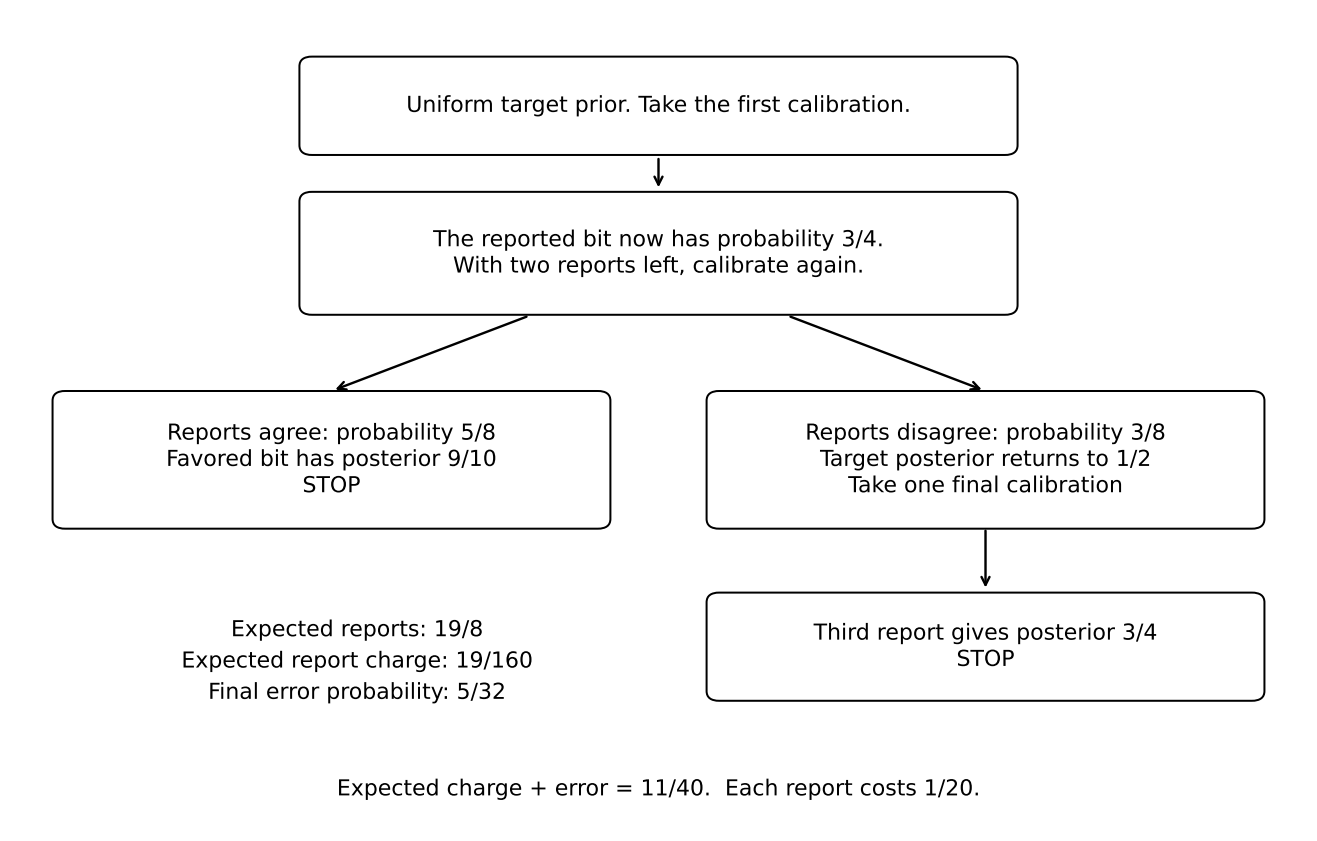
With three reports available, the optimal policy takes a second report after the first. If the first two agree, it stops. If they disagree, it takes the third. The disagreement probability is \(3/8\). Thus the expected report count is \(2+3/8=19/8\), the expected charge is \(19/160\), and the error probability is \(5/32\). The total is \(19/160+5/32=11/40\).
A horizon of two does not improve on one in this model: after the first result, paying for one additional report does not lower expected classification error enough to recover its charge. A horizon of three creates the option to investigate only the unresolved branch. The value comes from one contingent policy, not from separately optimal answers selected after the hidden bit is disclosed.
The two-valued predictive display state from Chapter 1 is too coarse for this inquiry. The four-pair probability record supports every calibration update and decision while still discarding the nuisance bit. This is the promised chain from evidence to representation to a useful experiment choice.
5.5 An approximate model supports a different, quantitative claim
On this page · Permalink · Source line 710
Exact policy transport and approximate planning must not share one unqualified guarantee. Fix a finite horizon \(H\) and one finite class \(\mathfrak P\) of admitted action/report trees, shared by the true and approximate models. The complete loss of a tree is the same function of its coarse-state and action/report path in both models, taking values in \([0,B]\). For example, a terminal loss in \([0,1]\) and at most \(H\) charges bounded by \(c_{\max}\) give \(B=1+Hc_{\max}\).
Assume Theorem 3.8's bound \(d_H\) holds uniformly over every tree in that class. An early stop is padded by a common absorbing terminal step for the history comparison. State-dependent charges are permitted when included in the same coarse-path loss. A model-dependent posterior score used as an uncharged surrogate loss would be a different problem.
Proposition 5.6: Uniform model error controls a changed policy
Let \(J(\pi)\) and \(\widetilde J(\pi)\) be a tree's expected losses in the true and approximate models. Then
If \(\widetilde\pi\) minimizes the approximate loss and \(\pi_*\) minimizes the true loss over this same class, then
These conclusions do not certify a zero-risk constraint or preservation of admissibility outside the common class.
Read proof · Recorded Lean scope · Permalink · Source line 715
Proof
The expectation of a function in \([0,B]\) changes by at most \(B\) times total variation. Apply the common-policy history bound separately to each fixed tree, proving the first assertion uniformly. Now
The range of loss gives the cap \(B\). The proof compares each tree with itself across the models before using the optimality inequality. It never applies a same-policy bound directly to two different controllers. A bad event assigned probability zero in one model can have small positive probability in the other, so an average bound supplies no sure-feasibility conclusion.
Source relationship. Direct combination of the newly admitted whole-history bound with the selection argument already used in Theorem 4.1; [AVOC], Sections 8–10, provide the source context for guarded planning and model-error value bounds. This finite fixed-policy-class formulation is stated and proved in full here.
With true calibration accuracy \(37/50\) and planning accuracy \(3/4\), the one-step defect is \(1/100\). For \(H=3\) and \(B=23/20\), the uniform regret bound is \(69/1000\). Exact observed performance is reported separately, not substituted for this guarantee. Expected-risk and hard-budget checks remain distinct. Next we study changes to the compiler producing the inquiry.