
11 Numerical evidence and applications
On this page · Permalink · Source line 1
Exact-law controls test values against independent formulas. Heterogeneous spectra test inversion across irregular coefficients. Simulated kernels test the operator pipeline. Timing measurements characterize particular implementations. These are distinct forms of evidence. The source package records the inputs and environments behind the reported experiments. The release regression and containment checks are reported in Appendix C.
11.1 Deep-tail controls
On this page · Permalink · Source line 10
A directed enclosure includes rounding as well as analytic remainders. An analytic ledger evaluated in ordinary floating point does not. The labels in this chapter identify which conclusion a result supports. The retained timing measurements are not presented as a new hardware comparison.
The method is designed for a regime in which direct survival probabilities can underflow long before the mathematical probability becomes numerically unresolvable. The engine therefore treats \(\log p\) as the primary numerical quantity and evaluates its error bounds on that logarithmic scale.
The validation ladder spans seven qualitatively different settings:
| validation regime | deepest \(\log_{10}p\) | observed error | certificate | spectral size |
|---|---|---|---|---|
| directed-rounding \(0.02\chi^2_{80}\) control | \(-5000\) | enclosure width \(3.34\times10^{-11}\) decades | multiplicative ratio \(\le 1+7.70\times10^{-11}\) | 80 df |
| large-scale positive spectrum | \(-922.031162\) | below stored reference resolution | \(5.71\times10^{-9}\) | rank 1997 |
| strong-dependence kernel | \(-457.973916\) | below stored reference resolution | \(5.20\times10^{-9}\) | rank 996 |
| heterogeneous inversion benchmark near \(10^{-16}\) | \(-16\) | \(2.88\)–\(6.52\times10^{-15}\) decades | independent integral converged | ranks 80–120 |
| signed finite-endpoint exact control | \(-200\) | \(\le 2.84\times10^{-14}\) decades | \(7.23\times10^{-13}\) | rank 80 |
| signed mixed multiscale | \(-81.891937\) | \(1.42\times10^{-12}\) decades vs full grid | \(5.78\times10^{-9}\) | rank 340 |
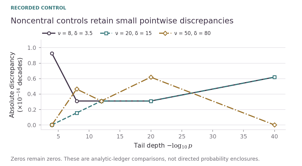
| noncentral exact controls | \(-40\) | \(\le 9.26\times10^{-15}\) decades | passing | up to 50 df |
The analytic scaled-chi-square ladder also includes
with respective reported absolute log-probability discrepancies
in the stored benchmark output. The corresponding analytic relative certificates remain finite throughout, reaching only
at \(10^{-5000}\).
A large-scale run with \(n=2000\), \(m=50{,}000\), 49,951 retained features, and quadratic-form rank 1997 produced
using 79 spectral packets and \(N=128\). Its independently evaluated full-spectrum tilted reference agreed within the stored reporting precision, while the reported relative certificate was
The corrected strong-dependence case study independently reached
with a finite \(5.20\times10^{-9}\) certificate. The signed finite-endpoint control passed its analytic ledger through \(10^{-200}\), while a rank-340 mixed-sign multiscale spectrum passed its analytic ledger to
Finally, the noncentral engine matched exact noncentral-chi-square controls from \(10^{-4}\) through \(10^{-40}\), with maximum observed discrepancy
decades.

11.1.1 Independent characteristic-function inversion near \(10^{-16}\)
On this page · Permalink · Source line 99
Closed-form controls are important, but they can hide numerical difficulties that appear only for heterogeneous spectra. An independent inversion test was therefore run on four generalized chi-square laws near
The reference evaluates the original characteristic function directly through the central Imhof inversion identity
where, for distinct positive coefficients \(\lambda_j\) with multiplicities \(h_j\),
This route does not use exponential tilting, the COS expansion, spectral packets, or the K-COS error controller.
The four spectra include balanced, skewed, dominant-spike, and higher-rank cases. Each reference integral was evaluated at two truncation limits. The omitted integral after the frequency cutoff \(T>0\) was bounded using
| spectrum | rank | \(|\Delta\log_{10}p|\) | relative difference | reference tail bound / \(p\) |
|---|---|---|---|---|
| balanced | 80 | \(6.52\times10^{-15}\) | \(1.50\times10^{-14}\) | \(6.84\times10^{-20}\) |
| skewed | 80 | \(4.13\times10^{-15}\) | \(9.50\times10^{-15}\) | \(4.44\times10^{-18}\) |
| spiky | 80 | \(5.19\times10^{-15}\) | \(1.20\times10^{-14}\) | \(7.00\times10^{-17}\) |
| balanced | 120 | \(2.88\times10^{-15}\) | \(6.64\times10^{-15}\) | \(4.19\times10^{-29}\) |
The two inversion truncations agree to between approximately
decades across the four cases. Thus the slow reference is numerically stable at a scale well below the observed K-COS-versus-inversion difference. Agreement between truncations is convergence evidence. The omitted-integral bound alone does not enclose quadrature discretization or numerical rounding, so this comparison is not assigned the directed-enclosure guarantee.

This test is complementary to the exact scaled-chi-square controls. It asks whether the solver remains accurate when no single-gamma reduction is available and when an algorithmically different inversion of the full characteristic function is used as the reference.
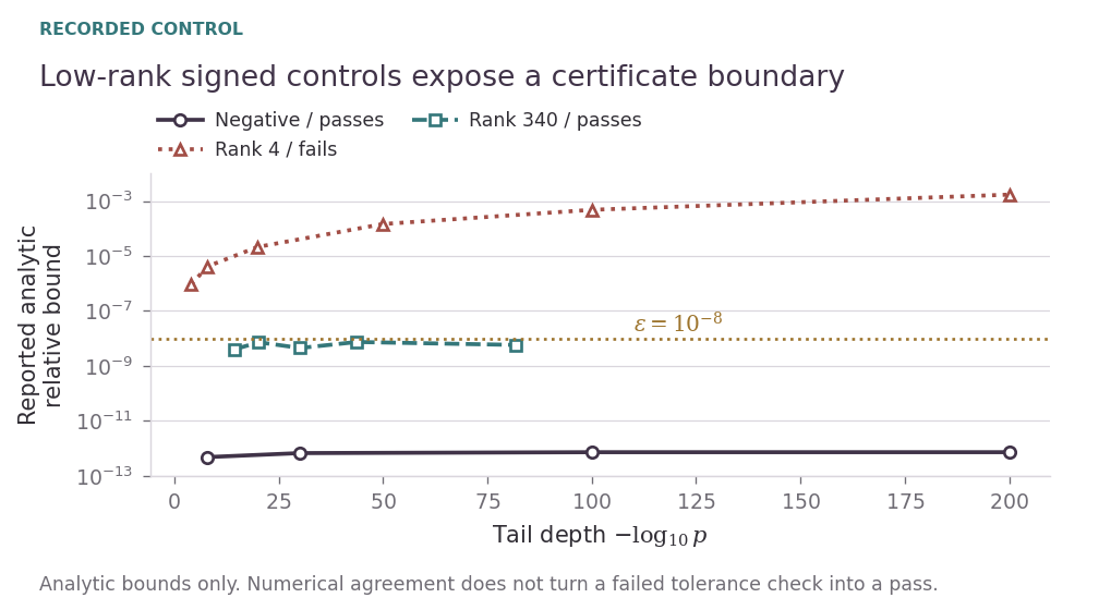
These results have different evidentiary roles. The scaled-chi-square, finite-endpoint signed, Laplace signed, and noncentral cases provide analytic controls. The heterogeneous inversion battery, large-scale, strong-dependence, and rank-340 mixed-sign cases test irregular spectra for which no single-gamma closed form is available. Together they test correctness against known distributions, representation compression, and stability on the intended high-rank numerical regime. The low-rank Laplace example also records a deliberate certificate failure boundary rather than conflating numerical agreement with certification.
11.2 Signed and noncentral controls
On this page · Permalink · Source line 198
Exact finite-endpoint control.
On this page · Permalink · Source line 199
For
the right tail is a lower chi-square tail with finite upper endpoint zero. The signed engine agrees with the exact distribution through
with maximum observed log-probability error about \(2.84\times10^{-14}\) decades and certificates around \(10^{-12}\).
Mixed-sign high-rank analytic-ledger control.
On this page · Permalink · Source line 212
A deterministic rank-340 multiscale spectrum with 180 positive and 160 negative coefficients was tested from approximately \(10^{-14}\) to
At the deepest point the packetized solver used 35 packets, \(N=4096\), and reported a relative certificate
Its log-probability differed from the unpacketized full-spectrum signed solver by about \(1.42\times10^{-12}\) decades. Independent exponential-tilt importance sampling placed the discrepancy at about \(1.41\) Monte Carlo standard errors.
Retained low-rank limitation.
On this page · Permalink · Source line 228
For independent \(Y_1,Y_2\sim\chi^2_2\), the quadratic form
is Laplace distributed with scale \(0.14\), so for \(q\ge0\),
The computed values agree with this exact law through \(10^{-200}\) to roughly \(10^{-9}\) decades or better. However, the implemented analytic COS-series certificate rejects these low-rank mixed cases because the tilted characteristic function decays only as \(|t|^{-2}\). The implementation reports this as a certificate failure rather than silently accepting the numerical value.
11.3 Rare-variant kernel case study
On this page · Permalink · Source line 260
The preceding sections establish operator identities and certified numerical bounds. This section tests the same machinery on the project's existing rare-variant SKAT simulation layer, including explicit LD structure, covariates, per-variant standardization, rare-variant weighting, and the phenotype-space score statistic.
11.3.1 Simulation provenance and implementation correction
On this page · Permalink · Source line 268
Two established genotype generators were used.
The first is a latent-Gaussian block-LD generator. Within a genomic block, alleles are obtained by thresholding correlated Gaussian latent variables at variant-specific minor-allele frequencies.
The second is a copy-LD generator in which haplotype states persist along a block with high probability and are occasionally redrawn. The simulator must initialize its genotype accumulator to zero before adding haplotypes. Allocating the accumulator with np.empty and then applying += would make the output depend on unspecified memory contents. All copy-LD results reported here use explicit zero initialization. Results from an uninitialized accumulator are excluded from the evidence record.
11.3.2 Tested LD regimes
On this page · Permalink · Source line 284
Four deterministic scenarios were evaluated.
| scenario | \(n\) | \(m\) | rank | median adjacent \(r^2\) | effective rank |
|---|---|---|---|---|---|
| latent LD, moderate | 600 | 3000 | 596 | 0.0069 | 441.9 |
| latent LD, strong | 600 | 3000 | 596 | 0.1140 | 240.3 |
| copy LD, strong | 600 | 3000 | 596 | 0.8298 | 200.1 |
| copy LD, large | 1000 | 5000 | 996 | 0.8179 | 353.0 |
Effective rank here is the participation ratio
It measures spectral concentration, not an integer count of nonzero directions. The corresponding spectra therefore span a substantial range of concentration: stronger LD reduces effective rank even when the nominal quadratic-form rank remains close to the sample residual dimension.

11.3.3 Streaming directly from raw genotype blocks
On this page · Permalink · Source line 320
The raw genotype matrix was streamed in resident variant blocks of widths 31, 127, and 509. Within each block the implementation performs
where \(\widetilde G_b\) denotes the centered and scaled block. The full weighted factor is never materialized.
Across all four LD scenarios and all three resident block sizes, the largest relative discrepancy against the fully materialized kernel was

This test is stronger than applying the streamed identity to a precomputed factor because the centering, variance scaling, covariate projection, and rare-variant weights are all performed inside the block loop.
11.3.4 Phenotype-space equivalence
On this page · Permalink · Source line 356
For each scenario, 100 Gaussian null residual draws were evaluated in three ways. Under the standardized Gaussian null, write \(e=M_Xz\) with \(z\sim N(0,I)\). Because \(M_XA=A\), the statistic used here is \(Q=\frac12 z^\top Kz\), so its nonzero mixture coefficients are \(\frac12\lambda_j(K)\). The factor \(\frac12\) belongs to this case-study normalization, not to the general quadratic-form definition.
directly through the factor,
\[ Q=\frac12\|A^\top e\|_2^2. \]through the sample kernel,
\[ Q=\frac12 e^\top Ke. \]through the eigencoordinates of \(K\).
The worst relative discrepancy across all draws and all scenarios was
Thus the simulated phenotype path, the streamed kernel, and the generalized \(\chi^2\) spectral representation agree to floating-point precision.
11.3.5 Deep tails on simulated LD spectra
On this page · Permalink · Source line 386
For every scenario, tail queries were generated at tilt fractions 0.90, 0.97, and 0.99 of the positive singularity. K-COS was compared with a higher-resolution full-spectrum tilted reference.
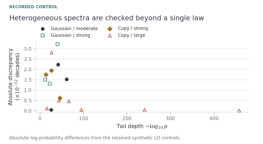
The large corrected copy-LD case was then pushed further, to fractions 0.995, 0.997, 0.999, and 0.9995. The deepest tested reference value was
At that point the displayed K-COS and high-resolution full-spectrum values were identical. Across the complete realistic-LD battery, the largest absolute discrepancy was
For the \(n=1000\), \(m=5000\) corrected copy-LD spectrum, selected results are
| tilt fraction | \(\log_{10}p\) | COS modes \(N\) | absolute error (decades) |
|---|---|---|---|
| 0.9950 | -65.950669 | 2048 | \(4.69\times10^{-13}\) |
| 0.9970 | -95.305034 | 2048 | \(3.70\times10^{-14}\) |
| 0.9990 | -240.602047 | 8192 | \(4.94\times10^{-14}\) |
| 0.9995 | -457.973916 | 16384 | below stored reference resolution |
11.3.6 Interpretation and boundary
On this page · Permalink · Source line 429
This simulation block does not add a new algebraic theorem. It supplies a more demanding validation layer for the theorem chain already proved. Specifically, it shows that the exact streaming identities and the K-COS deep-tail machinery remain numerically stable under substantially different rare-variant LD structures and through the complete raw-genotype preprocessing path.
The evidence remains synthetic. These generators do not reproduce every population-genetic feature of a sequencing cohort, and this block is not an external-cohort replication. It addresses the Gaussian linear-model null. Finite-sample Bernoulli or logistic calibration remains a separate statistical problem.
11.4 Spectral-packet experiments
On this page · Permalink · Source line 446
These tables and figures report the retained packet-planner experiments. Their analytic error bounds exclude floating-point roundoff. They measure a different numerical path from the directed positive backend, and are not reinterpreted as directed probability enclosures or new performance runs.
11.4.1 Exactly solvable chi-square stress test
On this page · Permalink · Source line 452
To isolate the effect of exponential tilting, we first used
whose survival probabilities are available directly from the chi-square distribution. Table 11.2 compares a global COS calculation with query-centered tilted COS.
| Target tail \(p\) | \(N\) | Global COS rel. error | Tilted COS rel. error |
|---|---|---|---|
| \(10^{-6}\) | 64 | \(3.56\times10^{-8}\) | \(2.71\times10^{-14}\) |
| \(10^{-10}\) | 64 | \(1.64\times10^{-4}\) | \(6.59\times10^{-15}\) |
| \(10^{-10}\) | 128 | \(2.03\times10^{-6}\) | \(9.05\times10^{-15}\) |
| \(10^{-14}\) | 64 | \(1.43\) | \(3.53\times10^{-14}\) |
| \(10^{-14}\) | 128 | \(6.15\times10^{-2}\) | \(3.87\times10^{-14}\) |
The test demonstrates the numerical motivation for tilting: evaluating a small tail directly under the shifted law is substantially more stable than reconstructing a global CDF and subtracting from one. This observation is not a novelty claim for exponential tilting itself.
11.4.2 Genotype-derived spectra
On this page · Permalink · Source line 479
The second experiment used the existing Komorebi SKAT benchmark generator. Synthetic genotype matrices were centered and scaled, then residualized against three covariates. The kernel weights were \(w_j=(1-\mathrm{MAF}_j)^{24}\), where MAF denotes minor-allele frequency. The factor used column scales \(\sqrt{w_j}\). Its positive quadratic-form spectrum was
Three independent \(n=400\), \(m=1200\) genotype sets yielded numerical rank \(397\). Four upper-tail queries per spectrum were generated by choosing saddlepoint locations at fractions \(0.70,0.80,0.85,0.90\) of the transform singularity. The comparison reference used exact-spectrum tilted COS with \(N=2048\) and a large support parameter \(L=20\). The adaptive method was asked for a relative analytic tolerance of \(10^{-8}\).
Across the twelve queries:
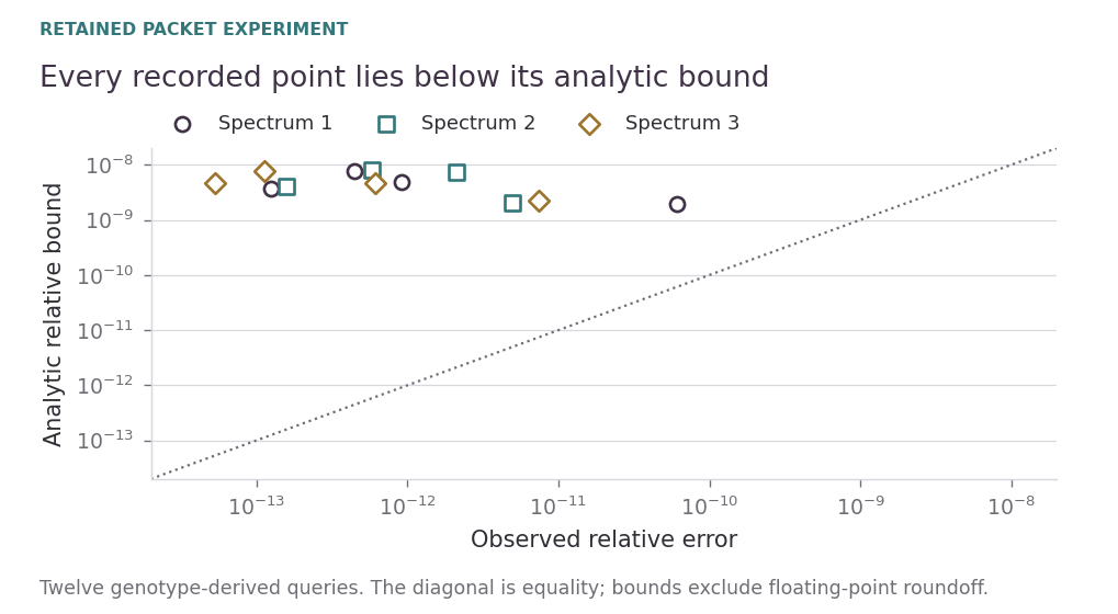
every requested \(10^{-8}\) analytic certificate passed.
the worst observed relative error was \(6.148608\times10^{-11}\).
the largest returned analytic relative bound was \(7.917203\times10^{-9}\).
the planner selected \(N\in\{64,128\}\), \(L\in\{10,11,12,13\}\), and 11–16 packets.
Figure 11.8 plots the observed errors against the returned analytic bounds. Every point lies above the equality line because the vertical coordinate is the bound.
11.4.3 Tolerance ladder
On this page · Permalink · Source line 504
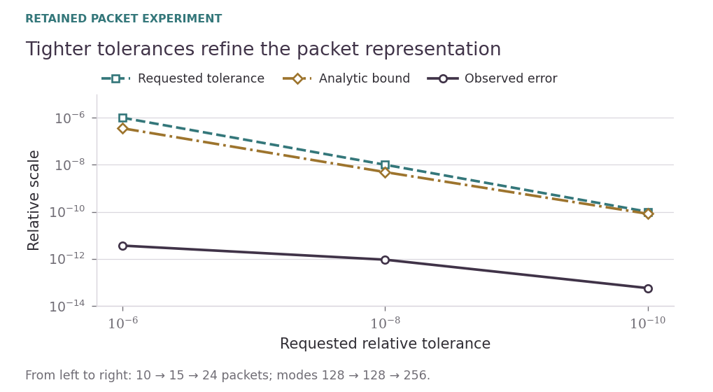
At a reference tail probability near \(8.99\times10^{-15}\), the same engine was requested to meet three tolerances. Table 11.3 shows how the representation refined automatically.
| Requested \(\tau\) | \(N\) | \(L\) | Packets | Analytic bound | Observed error |
|---|---|---|---|---|---|
| \(10^{-6}\) | 128 | 10 | 10 | \(3.56\times10^{-7}\) | \(3.63\times10^{-12}\) |
| \(10^{-8}\) | 128 | 12 | 15 | \(4.87\times10^{-9}\) | \(9.14\times10^{-13}\) |
| \(10^{-10}\) | 256 | 14 | 24 | \(8.21\times10^{-11}\) | \(5.65\times10^{-14}\) |
11.4.4 Prototype runtime scaling
On this page · Permalink · Source line 530
Table 11.4 reports median CPU timings from the Python prototype. “Adaptive total” includes planning and analytic error checks. “Compiled evaluation” measures reuse of an already compiled spectral passport at the selected grid.
| Rank | Packets | Exact tilted | Adaptive total | Compiled eval. | Compiled speedup |
|---|---|---|---|---|---|
| 397 | 13 | 6.66 ms | 10.45 ms | 0.549 ms | \(12.1\times\) |
| 797 | 16 | 13.32 ms | 11.49 ms | 0.604 ms | \(22.0\times\) |
| 1197 | 17 | 21.52 ms | 11.24 ms | 0.651 ms | \(33.1\times\) |
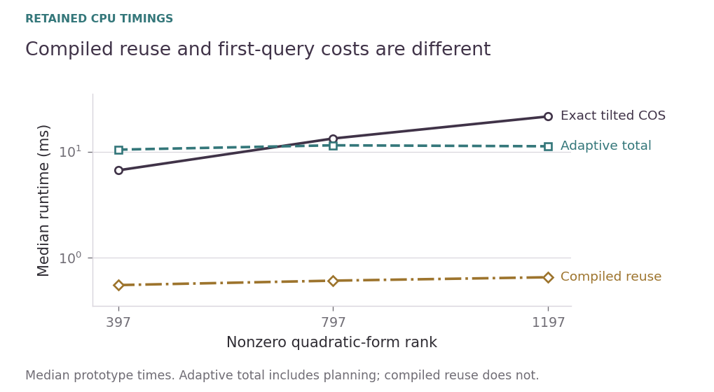
Planning matters. The first adaptive query is slower at rank 397 and faster at rank 797 in this prototype. Compiled reuse measures a different cost. These timings establish no universal speedup.
11.5 Numerical verification
On this page · Permalink · Source line 560
| partition | blocks | Gram relative error | action relative error |
|---|---|---|---|
| coarse 4 | 4 | \(2.91\times10^{-16}\) | \(5.99\times10^{-16}\) |
| fine 64 | 32 | \(3.39\times10^{-16}\) | \(6.00\times10^{-16}\) |
| irregular | 9 | \(3.34\times10^{-16}\) | \(5.87\times10^{-16}\) |
| singleton-front | 21 | \(2.43\times10^{-16}\) | \(5.82\times10^{-16}\) |
| permuted, block 73 | 29 | \(3.52\times10^{-16}\) | \(5.89\times10^{-16}\) |
Hierarchical refinement gave relative discrepancy \(3.17\times10^{-16}\). For \(H=L^\top L\) with block-bidiagonal \(L\), the smallest eigenvalue was approximately \(2.86\) and the largest norm outside the exact light cone was zero. The QR-core singular-spectrum discrepancy was \(5.89\times10^{-16}\) in relative \(\ell_2\) norm. These are finite controls, not universal floating-point error bounds.