
6 Exponential tilting and spectral packets
On this page · Permalink · Source line 1
The operator stage ends at a spectrum. The probability stage begins with a threshold and an accuracy requirement. Exponential tilting places the query in a better-conditioned region of the transformed law. Centered packets compress repeated transform evaluations on the grid that the query uses, without replacing the distribution by a moment-matched surrogate. Storage blocks partition a factor before eigendecomposition. Spectral packets group the coefficients after a spectrum is available. They act on different objects. The packet expansion approximates the transform on a specified complex grid and supplies a remainder bound on that grid.
The written packet bounds concern exact arithmetic. A directed packet implementation would also have to enclose its centers, moments, and transform evaluations. The positive interval backend in Chapter 9 instead evaluates the supplied spectrum directly. The two routes share the inversion analysis, but their arithmetic guarantees must not be conflated.
6.1 Quadratic-form transform and saddlepoint tilt
On this page · Permalink · Source line 15
Let
The variables \(Z_j\) are independent standard normal variables. The moment generating function exists for
and its cumulant generating function is
For complex \(s\), \(\kappa\) denotes the analytic logarithm normalized by \(\kappa(0)=0\). Each factor \(1-2s\lambda_j\) has positive real part on this domain, so its logarithm in the sum is principal. The sum need not equal the principal logarithm of the product, whose argument can wrap by \(2\pi\). For real \(\theta<1/(2\lambda_{\max})\),
At \(\theta=0\), this recovers the standard cumulant identity
Theorem 6.1: Unique upper-tail saddlepoint
If \(q>{\operatorname{\mathbb E}} Q=\sum_j\lambda_j\), there exists a unique
satisfying
Proof
By (6.3),
is continuous and strictly increasing on the stated interval. It equals \({\operatorname{\mathbb E}} Q\) at \(\theta=0\) and diverges as \(\theta\uparrow1/(2\lambda_{\max})\). The intermediate value theorem and strict monotonicity give existence and uniqueness.
Define the exponentially tilted law by
Its characteristic function is
and \({\operatorname{\mathbb E}}_{\theta}Q=\kappa'(\theta)\). Therefore the choice (6.4) moves the query \(q\) to the mean of the tilted law.
For any \(\theta>0\) in the transform domain,
This classical exponential-tilting identity lets K-COS evaluate the upper tail without subtracting a cumulative distribution function (CDF) value close to one.
6.2 Centered spectral packets
On this page · Permalink · Source line 97
Let a nonempty packet \(P\subset\{1,\ldots,r\}\) contain \(n_P\ge1\) eigenvalues. Define its center
and centered moments
Thus \(M_{P,0}=n_P\) and \(M_{P,1}=0\).
Theorem 6.2: Centered packet expansion
Fix \(s\in{\mathbb C}\) with \(\Re s<1/(2\lambda_{\max})\), use the principal logarithm, and define
For a nonnegative integer expansion order \(p\), if \(\rho_P(s)<1\), then the packet contribution to (6.2) is
where
Proof
For \(j\in P\),
The transform-domain condition gives positive real part for each \(1-2s\lambda_j\) and for \(1-2s\mu_P\). The disk condition gives positive real part for \(1-\alpha_P\delta_j\). The two factor arguments therefore sum inside \((-\pi,\pi)\), so their principal logarithms add without a branch ambiguity. Hence
When \(|\alpha_P\delta_j|<1\),
Summing over \(j\in P\) gives (6.10). The remainder satisfies
Using \(|z|\le\rho_P(s)\) and summing \(n_P\) terms yields (6.11).
Remark 6.3: What is compressed
A packet of \(n_P\) eigenvalues is replaced by its center and \(p\) centered moments. Large spectral spikes may be retained exactly. If the representation contains \(s\) exact eigenvalues and \(R\) packets of order \(p\), evaluation of the CGF on \(N\) frequencies costs \(O(N(s+R(p+1)))\) arithmetic operations after compilation, instead of \(O(Nr)\) direct eigenvalue-transform evaluations.
Remark 6.4: Query dependence
The relevant packet condition is not merely geometric closeness of eigenvalues. It is the complex-grid quantity \(\rho_P(\theta_*+{\mathrm{i}} u_k)\). Thus a partition suitable for one tail query or one COS grid need not be suitable for another.
6.3 The running example under an exponential tilt
On this page · Permalink · Source line 181
For spectrum \((1,1,2,2)\), the cumulant generator is \(\kappa(s)=-\log(1-2s)-\log(1-4s)\) on \(\Re s<1/4\). At \(q=40\), the saddlepoint equation reduces to \(160\theta^2-112\theta+17=0\), with
The other root lies outside the transform domain. The tilted mean is \(40\), while the likelihood-ratio identity restores the original tail probability.
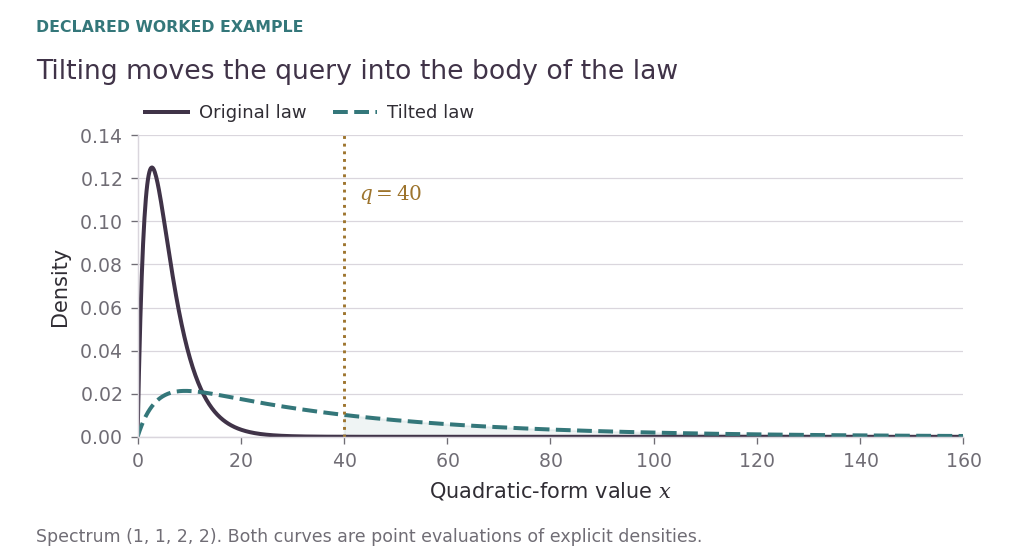
The two copies of \(1\) form one exact packet, and the two copies of \(2\) form another. All centered deviations vanish, so the packet remainder is zero on every admissible grid. The numerical enclosure still has support, Fourier-mode, and arithmetic errors.
6.4 A packet with a nonzero remainder
On this page · Permalink · Source line 203
To see the approximation itself, take a separate declared packet
and evaluate its contribution at \(s=0.1+0.4\,\mathrm i\). The deviations are \(-0.04,-0.02,0.02,0.04\). In particular,
The factor \(\alpha=2s/(1-4s)\) gives \(\rho=0.04|\alpha|<1\), so Theorem 6.2 applies. Retaining successive even moment orders gives the values below. Both columns are rounded point evaluations. The theorem, not these rounded comparisons, is the reason the remainder is bounded.
Permalink · Source line 204 · worked_packet_table.tex, line 1
| Order | Point-evaluated error | Analytic bound |
|---|---|---|
| 0 | \(2.3289\times10^{-4}\) | \(3.9366\times10^{-2}\) |
| 2 | \(3.6881\times10^{-8}\) | \(4.8893\times10^{-6}\) |
| 4 | \(8.7572\times10^{-12}\) | \(1.0931\times10^{-9}\) |
| 6 | \(2.419\times10^{-15}\) | \(2.9091\times10^{-13}\) |
| 8 | \(7.1896\times10^{-19}\) | \(8.4306\times10^{-17}\) |
| 10 | \(2.2307\times10^{-22}\) | \(2.5701\times10^{-20}\) |
