
Roots of unity, projectors, and falling-factorial coordinates
An extended hand-worked example · Komorebi P.
One polynomial will pass through a Fourier-style residue projector, a Newton/falling-factorial coordinate change, finite differences, exact shift-transfer blocks, and residue refinement. We will keep the objects and operations separate. In particular, we will see why projecting after a change of coordinates requires transporting the projector, not reusing its old formula.
The mathematical identities are classical: the roots-of-unity filter, Stirling inversion, Newton interpolation, umbral polynomial coordinates, and the forward difference. The purpose of this example is to exhibit their precise composition and recovery conditions in the realization-and-transfer language of the collection. No new theorem, Lean compilation, general analytic continuation, or novelty claim is made here.
Read the complete exact Python source · Download all source and results · Review the generated exact diagram
1. The destination: recover one ordinary power from three packets
Our fixed polynomial is
\[
f(x)=x^5.
\]
For a nonnegative integer \(k\), write the falling factorial
\[
x^{\underline{k}}=x(x-1)\cdots(x-k+1),
\qquad x^{\underline0}=1.
\]
The classical Stirling expansion reads
\[
\boxed{x^5
=x^{\underline1}+15x^{\underline2}
+25x^{\underline3}+10x^{\underline4}+x^{\underline5}.}
\]
We will separate those falling-factorial degrees into three congruence classes, then evaluate at \(x=4\).
The exact falling factorials at four are
| \(k\) | \(4^{\underline{k}}\) | \(S(5,k)\) | Weighted contribution |
|---|---|---|---|
| 0 | 1 | 0 | 0 |
| 1 | 4 | 1 | 4 |
| 2 | 12 | 15 | 180 |
| 3 | 24 | 25 | 600 |
| 4 | 24 | 10 | 240 |
| 5 | 0 | 1 | 0 |
Group the weighted contributions by \(k\bmod3\):
\[
\begin{aligned}
r=0:&\quad 25(24)=600,\\
r=1:&\quad 1(4)+10(24)=244,\\
r=2:&\quad 15(12)+1(0)=180.
\end{aligned}
\]
Therefore
\[
\boxed{600+244+180=1024=4^5.}
\]
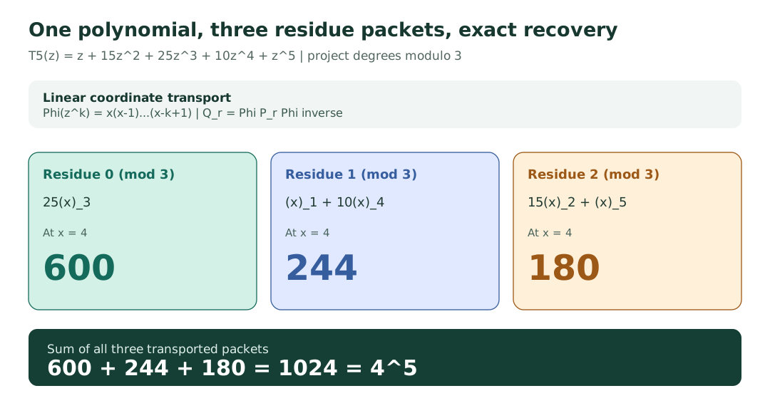
Download the complete coefficient and contribution table.
The remaining sections explain exactly which projector and coordinate map produce this calculation. They also exhibit a deliberately wrong operation.
The packets count actual functions
There is a completely different way to calculate the six contributions above. Let \(X\) have five elements and let \(Y\) have four labelled elements. Every function \(f:X\to Y\) uses some number \(k\) of distinct values in its image.
The number of functions with image size \(k\) is
\[
\boxed{\#\{f:X\to Y:\ |\operatorname{im}f|=k\}
=S(5,k)\,4^{\underline k}.}
\]
To see why, first partition the five input elements into \(k\) nonempty fibers, in \(S(5,k)\) ways. Then assign distinct labels from \(Y\) to those fibers, in \(4^{\underline k}\) ways. This assignment is bijective: every function specifies exactly its inverse-image partition and its fiber labels.
The exact image-size histogram is
\[
(k,\#f)=(0,0),(1,4),(2,180),(3,600),(4,240),(5,0).
\]
Grouping by \(k\bmod 3\) reproduces the three projected values \(600,244,180\). In the executable checker, this table is independently generated by enumerating all \(4^5=1024\) functions as actual five-tuples and counting distinct entries. That independent algorithm does not call the Stirling recurrence, Newton transform, or roots-of-unity projector.
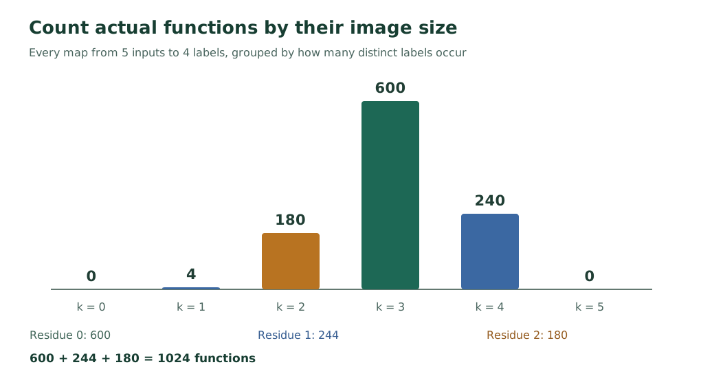
Download independently enumerated image-size histograms.
This answers a question the original three-packet calculation left implicit: the projector records the number of used output labels modulo three. It is not simply sorting powers of \(x\).
2. Roots of unity: project onto residue degrees
Work over the polynomial ring \(\mathbb Q(\zeta_m)[z]\), where \(m\ge2\) and \(\zeta_m\) is a primitive \(m\)-th root of unity. For each \(0\le r<m\), define
\[
\boxed{
P_r^{(m)}g(z)=\frac1m\sum_{\ell=0}^{m-1}
\zeta_m^{-r\ell}g(\zeta_m^\ell z).
}
\]
This expression is a finite sum of polynomials. There is no analytic convergence issue.
Apply the operator to a monomial:
\[
P_r^{(m)}z^k
=\left(\frac1m\sum_{\ell=0}^{m-1}
\zeta_m^{(k-r)\ell}\right)z^k
=\begin{cases}
z^k,&k\equiv r\pmod m,\\
0,&k\not\equiv r\pmod m.
\end{cases}
\]
The inner sum is either \(m\), or a geometric series whose ratio differs from one and whose sum is zero. Consequently, on rational polynomials the result has rational coefficients, despite the cyclotomic expression:
\[
P_r^{(m)}g(z)=
\sum_{k\equiv r\ (m)}[z^k]g(z)\,z^k.
\]
It follows immediately that
\[
P_rP_s=\delta_{rs}P_r,
\qquad
\sum_{r=0}^{m-1}P_r=I.
\]
These are complete, pairwise orthogonal algebraic projectors. Orthogonality here means \(P_rP_s=0\), not a claim about a particular inner product.
Exact check without floating-point roots. Let \(C\) be the cyclic permutation matrix of size \(m\). Its eigenvalues are precisely the \(m\)-th roots of unity and
\[
\frac1m\operatorname{tr}(C^{k-r})
=\begin{cases}1,&k\equiv r\pmod m,\\0,&\text{otherwise.}\end{cases}
\]
The standalone program verifies this equality using only integer counts of fixed coordinates of the cyclic permutation. This is an independent exact representation of the character filter, not a numerical evaluation of \(\zeta_m\).
3. The coordinate change is a linear map, not an algebra homomorphism
Define a \(\mathbb Q\)-linear map on polynomials by specifying its action on the monomial basis:
\[
\boxed{\Phi(z^k)=x^{\underline{k}}.}
\]
Because each falling factorial is monic of degree \(k\), this is a degree-preserving triangular linear isomorphism
\[
\Phi:\mathbb Q[z]\longrightarrow\mathbb Q[x].
\]
Do not read \(\Phi\) as evaluation at a particular \(z\). Its input and output variables name different coordinate descriptions.
The coefficients of the two triangular changes are the Stirling numbers:
\[
x^n=\sum_{k=0}^n S(n,k)x^{\underline{k}},
\]
and
\[
x^{\underline{k}}=\sum_{j=0}^k s(k,j)x^j,
\]
where \(s(k,j)\) are the signed Stirling numbers of the first kind. Therefore
\[
\boxed{\Phi^{-1}(x^n)=
\sum_{k=0}^nS(n,k)z^k.}
\]
For our fifth power,
\[
\Phi^{-1}(x^5)=
T_5(z)=z+15z^2+25z^3+10z^4+z^5,
\]
the fifth Touchard polynomial encountered in the Stirling, Bell and Fubini demonstration.
Why is the word linear essential? Consider
\[
\Phi(z)^2=x^2
\qquad\text{but}\qquad
\Phi(z^2)=x(x-1).
\]
Thus
\[
\boxed{\Phi(z^2)\ne\Phi(z)^2.}
\]
We cannot transport multiplication through \(\Phi\) while pretending the product in the target is unchanged. We will construct the correct transported product in Section 9.
4. Transport the projector into falling-factorial coordinates
The projector acting on the ordinary polynomial \(f(x)\) is
\[
\boxed{
Q_r^{(m)}=\Phi P_r^{(m)}\Phi^{-1}.
}
\]
For a polynomial expanded as
\[
f(x)=\sum_{k=0}^d a_kx^{\underline{k}},
\]
this becomes the explicit finite operation
\[
\boxed{
Q_r^{(m)}f(x)=
\sum_{\substack{0\le k\le d\\k\equiv r\pmod m}}
a_kx^{\underline{k}}.
}
\]
Because \(\Phi\) is invertible, the transferred operators obey
\[
Q_rQ_s=\delta_{rs}Q_r,
\qquad \sum_{r=0}^{m-1}Q_r=I.
\]
This is the original projector system transported to a new basis, not a new numerical approximation.
For \(f(x)=x^5\) and \(m=3\), the three packets are
\[
\begin{aligned}
Q_0f&=25x^{\underline3},\\
Q_1f&=x^{\underline1}+10x^{\underline4},\\
Q_2f&=15x^{\underline2}+x^{\underline5}.
\end{aligned}
\]
Expanding them in ordinary powers makes the change of basis visible:
\[
\begin{aligned}
Q_0f&=25x^3-75x^2+50x,\\
Q_1f&=10x^4-60x^3+110x^2-59x,\\
Q_2f&=x^5-10x^4+35x^3-35x^2+9x.
\end{aligned}
\]
All unwanted powers cancel in the sum, giving exactly \(x^5\).
There is also a concrete matrix formula. Let
\[
M_{i,k}=s(k,i),\qquad
(M^{-1})_{k,j}=S(j,k)
\]
be the linear coordinate matrices in ascending ordinary-power order. Then
\[
\boxed{
[Q_r]_{\text{power}}
=M\,D_r\,M^{-1},
\qquad
(D_r)_{k,k}=\mathbf1_{k\equiv r\pmod m},
}
\]
so that, for \(i\le j\),
\[
\boxed{
[Q_r]_{i,j}=
\sum_{\substack{i\le k\le j\\k\equiv r\pmod m}}
s(k,i)S(j,k).
}
\]
The source-bound matrix CSV gives all three \(6\times6\) rational matrices for degrees zero through five. The checker also verifies these entries directly against independently computed finite differences.
A valid projector that is wrong for this transfer
There is a typing distinction. The original \(P_r^{(m)}\) acts on polynomials in \(z\), while the transported \(Q_r^{(m)}\) acts on polynomials in \(x\). To compare operators on the same space, define the separate ordinary-power projector
\[
\widetilde P_r^{(m)}
\left(\sum_k c_k x^k\right)
=\sum_{k\equiv r\ (m)}c_kx^k.
\]
This is a valid family of complete, orthogonal projectors on \(\mathbb Q[x]\), but it is not the projector obtained by transporting \(P_r\) through \(\Phi\).
If we incorrectly substitute \(\widetilde P_r\) for \(Q_r\) in the falling-factorial calculation, we obtain
\[
\widetilde P_0^{(3)}x^5=0,\qquad
\widetilde P_1^{(3)}x^5=0,\qquad
\widetilde P_2^{(3)}x^5=x^5.
\]
At \(x=4\), this assigns all \(1024\) to residue two, whereas the correct transported packets give \((600,244,180)\). In particular,
\[
\boxed{(\widetilde P_2^{(3)}x^5)(4)=1024
\quad\ne\quad
(Q_2^{(3)}x^5)(4)=180.}
\]
Both projector systems are mathematically legitimate, and both act on \(\mathbb Q[x]\). They project different coordinate labels. The error is not the power-degree projector itself, but substituting it for the transported falling-factorial projector.
5. Newton differences give a second, independently computable inverse
Write the forward difference as
\[
(\Delta f)(x)=f(x+1)-f(x).
\]
For \(k\ge1\), the falling-factorial basis satisfies
\[
\boxed{\Delta x^{\underline{k}}
=kx^{\underline{k-1}}.}
\]
For \(k=0\), \(\Delta1=0\). Iterating, evaluating at zero, and using \(0^{\underline{k}}=0\) for \(k>0\) gives the exact Newton coefficient formula:
\[
\boxed{
a_k=\frac{(\Delta^kf)(0)}{k!},
\qquad
f(x)=\sum_{k=0}^{d}\frac{(\Delta^kf)(0)}{k!}
x^{\underline{k}}
}
\]
for any polynomial \(f\in\mathbb Q[x]\) of degree at most \(d\).
This can be proved without Stirling numbers. It also reconstructs the same Stirling coefficients when \(f(x)=x^n\):
\[
\begin{aligned}
(\Delta^k x^n)(0)
&=\sum_{j=0}^k(-1)^{k-j}\binom kj j^n\\
&=k!S(n,k).
\end{aligned}
\]
The second equality counts surjections onto \(k\) labelled targets by inclusion and exclusion; it uses \(0^0=1\) in the usual polynomial-evaluation convention.
For the fifth power, the Newton coefficients are
\[
\left(\frac{\Delta^k x^5(0)}{k!}\right)_{k=0}^5
=(0,1,15,25,10,1).
\]
Thus the same coefficients have three descriptions: the Stirling triangle, the inverse linear map \(\Phi^{-1}\), and differences at zero.
The general transported projector can now be written without introducing an auxiliary variable:
\[
\boxed{
Q_r^{(m)}f(x)=
\sum_{\substack{k\le\deg f\\k\equiv r\pmod m}}
\frac{(\Delta^kf)(0)}{k!}\,x^{\underline{k}}.
}
\]
This is a finite, executable formula for every rational polynomial.
An all-degree generating-function bridge
The same partition counts form a single exponential generating function. Let
\[
G_r^{(m)}(t,x)=\sum_{n\ge0}Q_r^{(m)}(x^n)\frac{t^n}{n!}.
\]
The classical fixed-\(k\) Stirling identity
\[
\sum_{n\ge0}S(n,k)\frac{t^n}{n!}
=\frac{(e^t-1)^k}{k!}
\]
immediately yields
\[
\boxed{
G_r^{(m)}(t,x)=
\sum_{\substack{k\ge0\\k\equiv r\pmod m}}
\binom{x}{k}(e^t-1)^k.
}
\]
Here \(\binom{x}{k}=x^{\underline k}/k!\) is a polynomial in \(x\). The series is understood formally in \(t\), with every coefficient a polynomial in \(x\). Thus no convergence at a numerical \(t\) is required.
Summing over all residue addresses gives
\[
\sum_{r=0}^{m-1}G_r^{(m)}(t,x)
=(1+(e^t-1))^x
=\boxed{e^{xt}},
\]
the EGF of \(x^n\). This identity is also the finite-function counting formula \(\sum_k S(n,k)x^{\underline k}=x^n\) simultaneously for every \(n\).
For the concrete integer codomain \(x=4\) and \(m=3\), put \(u=e^t-1\). Because \(\binom4k=0\) for \(k>4\),
\[
\begin{aligned}
G_0^{(3)}(t,4)&=1+4u^3,\\
G_1^{(3)}(t,4)&=4u+u^4,\\
G_2^{(3)}(t,4)&=6u^2.
\end{aligned}
\]
Extract the coefficient of \(t^5/5!\) and we recover, independently,
\[
\boxed{
5},G_1^{(3)},G_2^{(3)})
=(600,244,180).
}
\]
The exact program checks this formal-series identity coefficientwise through degree eight for integer and rational parameters \(x\) and moduli two, three, and four. Nonnegative integer values of \(x\) count functions. Other rational values remain valid polynomial identities, but are not assigned a literal finite-set counting interpretation.
Download the exact filtered EGF coefficients.
6. Transport differentiation: a cyclic finite-difference law
Let \(D_z=d/dz\). For \(k\ge1\), both operators lower their respective basis degrees in the same way:
\[
\Delta\Phi(z^k)
=kx^{\underline{k-1}}
=\Phi D_z(z^k).
\]
Both sides also vanish on the constant basis vector, since \(\Delta1=D_z1=0\). By linearity,
\[
\boxed{\Delta=\Phi D_z\Phi^{-1}.}
\]
Differentiation moves degree \(k\) to \(k-1\). Hence it moves residue \(r\) to \(r-1\), and
\[
\boxed{
\Delta Q_r^{(m)}
=Q_{r-1\pmod m}^{(m)}\Delta.
}
\]
In particular, \(\Delta^m\) commutes with every \(Q_r^{(m)}\).
For the fifth-power example, evaluate the differences of the three correct packets at \(x=4\):
| Original packet | Difference polynomial | Value at 4 | Target residue |
|---|---|---|---|
| \(Q_0f=25x^{\underline3}\) | \(75x^{\underline2}\) | 900 | 2 |
| \(Q_1f=x^{\underline1}+10x^{\underline4}\) | \(1+40x^{\underline3}\) | 961 | 0 |
| \(Q_2f=15x^{\underline2}+x^{\underline5}\) | \(30x^{\underline1}+5x^{\underline4}\) | 240 | 1 |
These add to
\[
900+961+240=2101=5^5-4^5
=(\Delta x^5)(4).
\]
The shift in packet address is part of the operator transfer. Comparing residues without that shift would conflate two different operations.
Download the finite-difference transfer table.
Spectral projectors from one backward-difference operator
The cyclic projectors admit another realization that needs neither complex roots nor an explicit Stirling-matrix inverse for each input.
Introduce the backward difference \(\nabla f(x)=f(x)-f(x-1)\). Define the transported degree operator
\[
\boxed{
\mathcal N=\Phi\left(z\frac{d}{dz}\right)\Phi^{-1}
=x\nabla.
}
\]
The second equality follows directly from
\[
x\nabla x^{\underline k}
=x\left(x^{\underline k}-(x-1)^{\underline k}\right)
=kx^{\underline k}.
\]
Thus the falling-factorial basis consists of \(\mathcal N\)-eigenvectors with eigenvalues \(k=0,1,2,\ldots\). This operator is not the ordinary Euler differential operator \(x\,d/dx\). For example,
\[
\boxed{
\mathcal N(x^2)=x(x^2-(x-1)^2)=2x^2-x
\ne 2x^2=x\frac{d}{dx}(x^2).
}
\]
On the finite-dimensional polynomial space \(V_d=\mathbb Q[x]_{\le d}\), define the usual rational Lagrange spectral factor
\[
L_{k,d}(\mathcal N)
=\prod_{\substack{0\le j\le d\\j\ne k}}
\frac{\mathcal N-jI}{k-j}.
\]
Its action on \(x^{\underline h}\) is \(\delta_{kh}x^{\underline h}\) for \(0\le h\le d\). Therefore
\[
\boxed{
Q_r^{(m)}\big|_{V_d}
=\sum_{\substack{0\le k\le d\\k\equiv r\pmod m}}
L_{k,d}(\mathcal N).
}
\]
This is a finite polynomial in the actual difference operator, with rational coefficients. The expression depends on the chosen degree bound \(d\); it is not claimed to be one finite-degree polynomial in \(\mathcal N\) valid on all of \(\mathbb Q[x]\).
We now have three exact descriptions of the same projector: a cyclotomic character average, conjugation by Stirling/Newton coordinates, and a rational spectral polynomial in \(x\nabla\). The checker constructs the third independently and compares its polynomial coefficients with the other descriptions.
A further compatibility identity is
\[
\boxed{
[\mathcal N,\Delta]=\mathcal N\Delta-\Delta\mathcal N=-\Delta,
}
\]
because on each basis vector \(x^{\underline k}\), the forward difference lowers the \(\mathcal N\)-eigenvalue by one. This supplies another algebraic explanation for the residue shift \(\Delta Q_r=Q_{r-1}\Delta\).
Download the rational spectral/projector comparison.
7. Translate the input and follow every cross-packet term
The earlier differentiation rule describes how a packet's degree decreases. We can now transport the whole shift, including its diagonal part and the terms crossing between residue classes.
Write
\[
(T_hf)(x)=f(x+h),\qquad h\in\mathbb Q.
\]
Falling factorials satisfy a binomial-type addition formula:
\[
\boxed{
(x+h)^{\underline k}=
\sum_{j=0}^k\binom kj
x^{\underline j}h^{\underline{k-j}}.
}
\]
Proof. Expand the formal identity
\[
(1+u)^{x+h}=(1+u)^x(1+u)^h
\]
using \((1+u)^x=\sum_{k\ge0}x^{\underline k}u^k/k!\) in \(\mathbb Q[x][[u]]\), and compare the coefficient of \(u^k/k!\). No convergence or evaluation at a complex argument is involved.
If \(f=\sum_k a_kx^{\underline k}\), this supplies every cross-packet transfer block:
\[
\boxed{
Q_r^{(m)}T_hQ_s^{(m)}f=
\sum_{\substack{k\equiv s\ (m)}}a_k
\sum_{\substack{0\le j\le k\\j\equiv r\ (m)}}
\binom kj h^{\underline{k-j}}x^{\underline j}.
}
\]
This expression works for rational \(h\), including negative and fractional steps. The corresponding source-to-target block matrix is not assumed to be diagonal.
An especially simple two-tap shift
At \(h=1\), the only nonzero falling factorials \(1^{\underline\ell}\) occur at \(\ell=0,1\). Hence
\[
T_1=I+\Delta
\]
and
\[
\boxed{
Q_r^{(m)}T_1Q_s^{(m)}
=\delta_{rs}Q_s^{(m)}
+\delta_{r,s-1\ (\mathrm{mod}\ m)}\Delta Q_s^{(m)}.
}
\]
For our three residue packets:
\[
\boxed{
\begin{pmatrix}
Q_0T_1f\\Q_1T_1f\\Q_2T_1f
\end{pmatrix}
=
\begin{pmatrix}
I&\Delta&0\\
0&I&\Delta\\
\Delta&0&I
\end{pmatrix}
\begin{pmatrix}Q_0f\\Q_1f\\Q_2f\end{pmatrix}.
}
\]
The off-diagonal difference operators are genuine transfers from one falling-degree residue into another.
At \(x=4\), compute each output packet independently:
| Target residue | Original \(Q_rf(4)\) | Carry from next residue | \(Q_r(T_1f)(4)\) | \((T_1Q_rf)(4)\) |
|---|---|---|---|---|
| 0 | 600 | \(\Delta Q_1f(4)=961\) | 1561 | 1500 |
| 1 | 244 | \(\Delta Q_2f(4)=240\) | 484 | 1205 |
| 2 | 180 | \(\Delta Q_0f(4)=900\) | 1080 | 420 |
| Total | 1024 | 2101 | 3125 | 3125 |
Both right-hand columns reconstruct \(5^5=3125\), but they label the components differently:
\[
(Q_0T_1f,Q_1T_1f,Q_2T_1f)(4)
=(1561,484,1080),
\]
whereas
\[
(T_1Q_0f,T_1Q_1f,T_1Q_2f)(4)
=(1500,1205,420).
\]
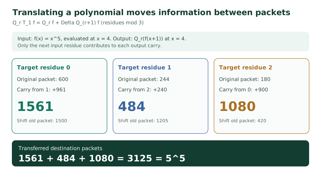
The discrepancy is a noncommutation witness, not numerical error. In fact,
\[
\boxed{
[Q_r^{(m)},T_1]f
=\Delta Q_{r+1}^{(m)}f-\Delta Q_r^{(m)}f
}
\]
and for the three packets its evaluation at four is
\[
\boxed{(61,-721,660),\qquad61-721+660=0.}
\]
The sum of the commutator packets vanishes because \(\sum_rQ_r=I\), even though individual commutators need not vanish.
Arbitrary integer steps and finite transfer bandwidth
When \(h\) is a nonnegative integer, \(h^{\underline\ell}=0\) for \(\ell>h\). Thus an input falling degree \(k\) can reach only degrees \(k,k-1,\ldots,k-h\). The \(m\times m\) residue transfer therefore has at most \(h+1\) allowed cyclic diagonals, possibly fewer when residues coincide. For instance, \(h=2\) requires three possible shifts rather than two.
Fractional or negative \(h\) need not have this fixed finite bandwidth: the connection formula is still a finite sum on each polynomial of fixed degree, but its number of potentially nonzero terms can grow with the degree.
The checker computes \(Q_rT_hQ_s\) from the falling-factorial binomial identity and, independently, by ordinary-power translation followed by the projector. It compares both through multiple moduli, polynomial degrees and rational shifts. A complete source-to-target table for \(h=0,1,2\) is downloadable.
Download the exact translation block matrix entries · Download the two different shifted packet ledgers.
The corresponding carry in the all-degree generating functions
The filtered generating functions from Section 5 satisfy a compatible identity. The formal binomial recurrence
\[
\binom{x+1}{k}=\binom{x}{k}+\binom{x}{k-1}
\]
implies, with \(u=e^t-1\),
\[
\boxed{
G_r^{(m)}(t,x+1)
=G_r^{(m)}(t,x)
+(e^t-1)G_{r-1}^{(m)}(t,x).
}
\]
This concerns evaluation of the original \(r\)-packet at the shifted argument. It corresponds to \(T_1Q_rf\), not to \(Q_rT_1f\). Those two operations must not be silently identified. For \(m=3,x=4,n=5\), its coefficient changes are \(900,961,240\), precisely the differences in the last numerical column above.
The checker verifies this formal-series carry equation coefficientwise for several integer and rational \(x\), not solely at \(x=4\).
8. Refine the same packets without changing their sum
The same congruence class modulo three splits into two disjoint classes modulo six:
\[
\boxed{
Q_r^{(3)}=Q_r^{(6)}+Q_{r+3}^{(6)},
\qquad r=0,1,2.
}
\]
On \(x^5\), the six child values at \(x=4\) are:
| Parent residue | Child \(r\) | Child \(r+3\) | Parent total |
|---|---|---|---|
| 0 | 0 | 600 | 600 |
| 1 | 4 | 240 | 244 |
| 2 | 180 | 0 | 180 |
The zeros are meaningful. The degree-zero coefficient of \(x^5\) is zero, and \(4^{\underline5}=0\).
More generally, if \(M\) is a multiple of \(m\),
\[
Q_r^{(m)}=
\sum_{q=0}^{M/m-1}Q_{r+mq}^{(M)}.
\]
This is exact address refinement, not an error-producing truncation. Discarding a child instead leaves the explicitly omitted polynomial, which can be evaluated or reconstructed exactly.
Download the refinement table.
9. Multiplication must also be transported
The linear change \(\Phi\) does not preserve ordinary polynomial multiplication. If we want multiplication in the Newton coordinate algebra to survive, define a transported product on \(\mathbb Q[x]\):
\[
\boxed{
f\star g=\Phi\bigl(\Phi^{-1}f\cdot\Phi^{-1}g\bigr).
}
\]
In particular,
\[
x^{\underline a}\star x^{\underline b}
=x^{\underline{a+b}},
\]
so
\[
x\star x=x(x-1)\ne x^2.
\]
This product is associative, commutative and unital because ordinary multiplication in \(\mathbb Q[z]\) has those properties. The transformed difference is a derivation for \(\star\):
\[
\boxed{
\Delta(f\star g)
=(\Delta f)\star g+f\star(\Delta g).
}
\]
Residue packets now multiply by cyclic convolution:
\[
\boxed{
Q_r^{(m)}(f\star g)
=\sum_{\substack{0\le a,b<m\\a+b\equiv r\pmod m}}
(Q_a^{(m)}f)\star(Q_b^{(m)}g).
}
\]
For comparison, ordinary pointwise multiplication satisfies the shifted finite-difference product rule
\[
\Delta(fg)=(\Delta f)g+f(x+1)(\Delta g).
\]
The naive differential Leibniz rule fails even for \(f=g=x\):
\[
\Delta(x^2)=2x+1\ne2x.
\]
This is a useful boundary example. We can transport an operation exactly, but the transported operation need not be identical to the familiar operation on the target coordinates.
10. General scope and conditions
A sharp characteristic-three obstruction
The distinction between coordinate transport and a particular spectral formula is even clearer over a finite field.
The linear transformation \(\Phi(z^k)=x^{\underline k}\) is unitriangular with integer Stirling coefficients and inverse. It remains an invertible change of polynomial basis over any commutative coefficient ring, including \(\mathbb F_3\). What fails in characteristic three is the difference quotient \(a_k=(\Delta^kf)(0)/k!\) for \(k\ge3\), not the existence of the falling-factorial basis itself.
Likewise, our rational Lagrange formula for spectral projectors divides by \(k-j\). In characteristic three, the operator \(\mathcal N=x\nabla\) has colliding eigenvalues:
\[
\begin{aligned}
v_0&=x^{\underline0}=1,&\quad\mathcal Nv_0&=0,\\
v_3&=x^{\underline3}=x^3-x\ne0,&\quad\mathcal Nv_3&=3v_3=0
\quad\text{in }\mathbb F_3[x].
\end{aligned}
\]
The polynomial \(x^3-x\) is nonzero in \(\mathbb F_3[x]\), even though it evaluates to zero at every point of \(\mathbb F_3\). This is an argument in the polynomial ring, not in the space of polynomial functions on \(\mathbb F_3\).
The coefficient projector by parity is still perfectly well defined: the order \(m=2\) is invertible modulo three and the root \(-1\) exists in \(\mathbb F_3\). This does not assert that the cyclotomic averaging formula works when the projector modulus is divisible by the characteristic. The parity projector acts as follows:
\[
\boxed{
Q_0^{(2)}v_0=v_0,\qquad Q_0^{(2)}v_3=0.
}
\]
Suppose, contrary to fact, that one polynomial \(H(\mathcal N)\) represented \(Q_0^{(2)}\) on all polynomials of degree at most three. Both \(v_0\) and \(v_3\) are nonzero eigenvectors with the same eigenvalue zero, so \(H(\mathcal N)\) acts on each as multiplication by \(H(0)\). The first required value forces \(H(0)=1\), while the second forces \(H(0)=0\). Contradiction.
Thus the projector survives, but its proposed realization as a polynomial in this single degree operator fails in that coefficient field. On degrees strictly below the characteristic, the distinct eigenvalues permit the usual Lagrange construction; the collision becomes unavoidable at degree three for this example.
There is a parallel finite-difference obstruction: over \(\mathbb F_3[x]\),
\[
\boxed{\Delta^3=(T_1-I)^3=T_3-I=0.}
\]
The equality uses characteristic three and \(T_3f(x)=f(x+3)=f(x)\). Consequently, high-order differences cannot recover all falling-factorial coefficients by division. The integral Stirling matrix inverse still does.
This is a deliberate negative control against extending a rational spectral argument across a characteristic boundary without checking its denominators and eigenvalue separation.
Download the exact characteristic-three obstruction.
Except for the explicitly identified characteristic-three example, the constructions above are exact for polynomials over \(\mathbb Q\), with projector modulus \(m\ge2\). The function-counting interpretation additionally requires nonnegative integer domain and codomain sizes, whereas the packet EGF and rational spectral projector identities do not.
- The roots-of-unity formula uses a field containing \(m\)-th roots of unity and an invertible \(m\), but its output on \(\mathbb Q[z]\) is rational.
- The Newton difference-quotient formula divides by \(k!\) and does not transfer unchanged when that factorial is not invertible. The integral, unitriangular Stirling basis isomorphism remains valid over any commutative coefficient ring. By contrast, the finite-degree Lagrange spectral formula requires the eigenvalue differences used in its denominators to be units. The characteristic-three example distinguishes these facts.
- For functions on the nonnegative integers, Newton's formula recovers each fixed value through a finite sum up to that index. The polynomial isomorphism statement does not imply arbitrary analytic, \(p\)-adic, or infinite-series convergence.
- The forward difference is the transported derivative. Ordinary differentiation \(d/dx\) is a different operation. The backward difference, multiplied by \(x\), realizes the transported degree operator. Its finite Lagrange projector formula depends on the degree bound.
- The transported product \(\star\) is not ordinary multiplication. Claims about multiplicative transport must name the product they use.
The program tests the general finite identities, not merely the displayed numerical example. It checks independent Stirling/finite-difference coefficient routes, inverse triangular matrices, idempotence and orthogonality, exact cyclic traces for moduli two through six, operator conjugation in ordinary-power matrices, finite-difference and general translation transfers, refinements, transported multiplication, the rational spectral formula, exhaustive function enumeration, filtered formal EGFs, explicit modular basis-inversion and characteristic-three difference controls, and deliberately invalid operator substitutions.
No assertion about an unrelated arithmetic conjecture follows from these finite polynomial identities.
11. Run, inspect, and reproduce
The complete Python program needs only Python 3.10 or later and its standard library. No network, symbolic algebra dependency, complex floating arithmetic, or random inputs are required.
From the repository root:
python -B examples/roots_unity_falling_factorial.py
python -B examples/roots_unity_falling_factorial.py --output roots-results
The first command performs the exact checks and prints the three-packet reconstruction and shift-transfer comparison. The second also writes eleven exact CSV tables, three accessible Python-generated SVG diagrams, and a JSON summary. Existing output files are not overwritten. The publisher recreates the same files on the website and binds their hashes to the committed program and manuscript.
Source-and-results ZIP · Python source · Source identity record · Exact results (JSON)
The previous work this example connects
- Factorial lanes gives the general cyclotomic coefficient projector and distinguishes additive residue packets from multiplicative step-factorial lanes.
- Euler numbers through packets develops Newton/Pascal coordinate transformations, conjugated sampling, prime-sensitive difference estimates, and their genuine analytic boundaries.
- Stirling, Bell and Fubini develops the triangular inversion, formal exponential substitution, and coupled roots-of-unity packets.
- Wavelets and polyphase transfer illustrates the same requirement to transport the operation, including cross-channel terms that disappear in invalid shortcuts.
- Paper IV, Paper IX, and Special Functions provide the corresponding broader research contexts, each with its own hypotheses and verification evidence.
This calculation is intentionally a finite polynomial bridge. It does not import the proof status of those other works or claim to resolve their remaining questions.