
From set partitions to exact transfer: Stirling, Bell and Fubini numbers
An extended hand-worked example · Komorebi P.
One triangular table counts partitions of labelled objects into nonempty blocks. Constant and factorial weights on that same table generate Bell and ordered Bell (Fubini) numbers. We compute both from an explicit row, prove the general generating-function substitution and its inverse, trace polynomial and moment realizations, and identify the boundary between reversible data and lossy summaries.
No new mathematical result is claimed. The counting identities are classical. The purpose is to follow one explicit object through the coordinate, transfer, reconstruction and obstruction language used throughout the collection.
Run the existing factorial-weight experiment · Read the exact program · Download the verified results
The destination: two answers from the same partition row
Let \(S(n,k)\) be the Stirling number of the second kind: the number of partitions of an \(n\)-element labelled set into exactly \(k\) nonempty, unlabelled blocks. Set \(S(0,0)=1\), and let entries outside \(0\le k\le n\) be zero.
Our central object is
\[
\boxed{
(S(5,0),S(5,1),\ldots,S(5,5))
=(0,1,15,25,10,1).
}
\]
Adding these coordinates counts partitions without ordering the blocks:
\[
\boxed{B_5=0+1+15+25+10+1=52.}
\]
A partition with \(k\) blocks can have those blocks ordered in \(k!\) ways. The same row, with its \(k\)-th coordinate multiplied by \(k!\), becomes
| Blocks \(k\) | Partitions \(S(5,k)\) | Block orders \(k!\) | Ordered contributions \(k!S(5,k)\) |
|---|---|---|---|
| 0 | 0 | 1 | 0 |
| 1 | 1 | 1 | 1 |
| 2 | 15 | 2 | 30 |
| 3 | 25 | 6 | 150 |
| 4 | 10 | 24 | 240 |
| 5 | 1 | 120 | 120 |
| Sum | 52 | 541 |
Thus
\[
\boxed{F_5=\sum_{k=0}^5 k!S(5,k)=541.}
\]
Here \(B_n\) denotes the Bell numbers and \(F_n\) denotes the ordered Bell, or Fubini, numbers. Some sources use a different symbol for \(F_n\); we use \(F\) consistently on this page.
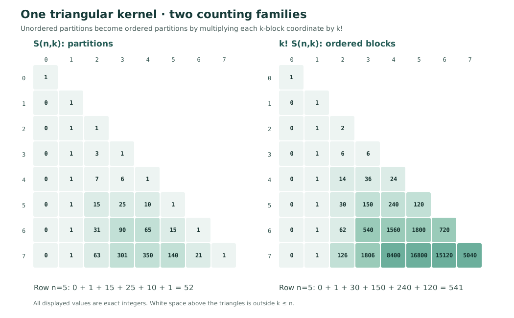
The image is produced by the standalone Python program. Every cell is an exact integer, not a logarithmically rounded coefficient. The complete table is available as CSV.
1. Construct the triangular coordinates
For example, a three-element set has exactly three partitions into two nonempty blocks: \(\{1\}\mid\{2,3\}\), \(\{2\}\mid\{1,3\}\), and \(\{3\}\mid\{1,2\}\). Hence \(S(3,2)=3\).
To make a partition of \(\{1,\ldots,n\}\) into \(k\) blocks, inspect the last element \(n\).
It either forms a singleton block, leaving a partition of \(n-1\) objects into \(k-1\) blocks, or joins one of \(k\) blocks of a partition of \(n-1\) objects into \(k\) blocks. Therefore
\[
\boxed{S(n,k)=S(n-1,k-1)+kS(n-1,k).}
\]
Starting with \(S(0,0)=1\), this gives:
| \(n\) | \(S(n,0),\ldots,S(n,n)\) | \(B_n\) | \(F_n\) |
|---|---|---|---|
| 0 | \(1\) | 1 | 1 |
| 1 | \(0,1\) | 1 | 1 |
| 2 | \(0,1,1\) | 2 | 3 |
| 3 | \(0,1,3,1\) | 5 | 13 |
| 4 | \(0,1,7,6,1\) | 15 | 75 |
| 5 | \(0,1,15,25,10,1\) | 52 | 541 |
| 6 | \(0,1,31,90,65,15,1\) | 203 | 4683 |
For example, \(S(5,3)=S(4,2)+3S(4,3)=7+3(6)=25\). The triangular recurrence determines the complete row with no numerical approximation.
We distinguish this recurrence from the site’s finite residue-packet and FIR-filter examples: the Stirling triangle is a triangular transformation across different sequence indices, not a fixed-length translation-invariant convolution.
2. Make the operator explicit
Let \(\mathcal S\) be the infinite lower-triangular matrix
\[
\mathcal S_{nk}=S(n,k),\qquad n,k\ge0.
\]
If the input weights are \(a_k\), the output family is
\[
\boxed{(\mathcal Sa)_n=\sum_{k=0}^n S(n,k)a_k.}
\]
For our two examples,
\[
\begin{aligned}
a^{\mathrm B}&=(1,1,1,1,\ldots),
&\mathcal Sa^{\mathrm B}&=(B_0,B_1,B_2,\ldots),\\
a^{\mathrm F}&=(0!,1!,2!,3!,\ldots),
&\mathcal Sa^{\mathrm F}&=(F_0,F_1,F_2,\ldots).
\end{aligned}
\]
Equivalently, write \(D=\operatorname{diag}(0!,1!,2!,\ldots)\). The two maps are \(\mathcal S\) and \(\mathcal SD\) acting on the constant sequence \(\mathbf1\). All finite truncations of \(\mathcal S\) have diagonal entries \(S(n,n)=1\), and hence determinant one. The diagonal \(D\) is invertible over \(\mathbb Q\), although \(D^{-1}\) contains reciprocal factorials.
Here are the first five rows, with columns indexed from zero:
\[
\mathcal S_{0:4}
=\begin{pmatrix}
1&0&0&0&0\\
0&1&0&0&0\\
0&1&1&0&0\\
0&1&3&1&0\\
0&1&7&6&1
\end{pmatrix}.
\]
Applying it to \((1,1,1,1,1)^{\mathsf T}\) gives \((1,1,2,5,15)^{\mathsf T}\), while applying it to \((1,1,2,6,24)^{\mathsf T}\) gives \((1,1,3,13,75)^{\mathsf T}\).
One kernel, different inputs, different families. The choice of weight sequence is mathematical data, not an arbitrary display setting.
3. Undo the transfer exactly
Let \(s(n,k)\) denote the signed Stirling numbers of the first kind, defined by
\[
x(x-1)\cdots(x-n+1)=\sum_{k=0}^n s(n,k)x^k.
\]
They satisfy \(s(0,0)=1\) and
\[
s(n,k)=s(n-1,k-1)-(n-1)s(n-1,k).
\]
Why this is the inverse: for a positive integer \(x\), count all functions from an \(n\)-element set into an \(x\)-element set. Every function determines a partition into its \(k\) nonempty inverse-image blocks. After choosing that partition, there are \(x(x-1)\cdots(x-k+1)\) ways to assign distinct target labels to its blocks. Thus
\[
x^n=\sum_{k=0}^n S(n,k)\,x(x-1)\cdots(x-k+1).
\]
The identity holds as a polynomial because it holds for every positive integer \(x\). Substitute the signed first-kind polynomial expansion and compare powers of \(x\). This gives \(\mathcal S\,s=I\). Both matrices are lower triangular with diagonal one, so the reverse product is also \(s\,\mathcal S=I\) in every finite truncation.
The two triangular matrices are inverses:
\[
\boxed{\sum_{j=k}^n s(n,j)S(j,k)=\delta_{nk},
\qquad
\sum_{j=k}^n S(n,j)s(j,k)=\delta_{nk}.}
\]
Thus knowing the complete sequence \((B_0,\ldots,B_n)\) recovers its original weight at \(n\), and similarly for Fubini:
\[
\sum_{j=0}^n s(n,j)B_j=1,
\qquad
\sum_{j=0}^n s(n,j)F_j=n!.
\]
For \(n=5\), the inverse coefficients are
\[
(s(5,0),\ldots,s(5,5))=(0,24,-50,35,-10,1).
\]
The Fubini inverse works by direct arithmetic:
\[
24(1)-50(3)+35(13)-10(75)+541
=24-150+455-750+541
=\boxed{120=5!}.
\]
The Bell inverse gives
\[
24(1)-50(2)+35(5)-10(15)+52
=\boxed{1}.
\]
This inversion is not reconstructing an arbitrary Stirling row from just one Bell or Fubini value. It inverts the known triangular transform across the sequence of all preceding output indices.
Inspect the signed transfer matrix and its exact identity product.
4. Generate both families from exponential series
A second derivation checks the same arithmetic by an independent route. There are \(k!S(n,k)\) onto maps from an \(n\)-element set to \(k\) labelled targets. Inclusion and exclusion give
\[
k!S(n,k)
=\sum_{j=0}^k(-1)^{k-j}\binom{k}{j}j^n.
\]
For fixed \(k\), sum over \(n\) as an exponential generating function:
\[
\begin{aligned}
\sum_{n\ge0} S(n,k)\frac{t^n}{n!}
&=\frac1{k!}\sum_{j=0}^k(-1)^{k-j}\binom{k}{j}e^{jt}\\
&=\boxed{\frac{(e^t-1)^k}{k!}}.
\end{aligned}
\]
Set \(u(t)=e^t-1\), which has zero constant term. Reweighting this identity yields two distinct generating functions:
\[
\begin{aligned}
\sum_{n\ge0}B_n\frac{t^n}{n!}
&=\sum_{k\ge0}\frac{u(t)^k}{k!}
=\boxed{\exp(e^t-1)},\\[2mm]
\sum_{n\ge0}F_n\frac{t^n}{n!}
&=\sum_{k\ge0}u(t)^k
=\boxed{\frac1{2-e^t}}.
\end{aligned}
\]
These are exact identities of formal power series over \(\mathbb Q\). The sums are well defined coefficient by coefficient because \(u(t)^k\) starts at degree \(k\). No analytic convergence assumption is needed for the formal identities.
This makes the connection to the Euler and factorial-lane demonstrations precise: the Fubini generating function is another reciprocal series, but its denominator and indexing are different. The resulting coefficient family is not the Euler sequence.
The general input rule and its formal inverse
The two generating functions above are instances of a single, exact operation. For an arbitrary weight sequence \(a_0,a_1,\ldots\) over \(\mathbb Q\), write
\[
c_n=\sum_{k=0}^n S(n,k)a_k,\qquad
A(u)=\sum_{k\ge0}a_k\frac{u^k}{k!},\qquad
C(t)=\sum_{n\ge0}c_n\frac{t^n}{n!}.
\]
Substitute the fixed-\(k\) identity from the start of this section, rearranging only coefficientwise finite sums:
\[
\boxed{C(t)=A(e^t-1).}
\]
The inverse substitution exists because \(e^t-1\) has zero constant term and linear coefficient one. Its compositional inverse is \(\log(1+u)\). Therefore
\[
\boxed{A(u)=C(\log(1+u)).}
\]
This is the formal-series counterpart of the signed-Stirling matrix inversion in Section 3. The two inversion methods act in different coordinate descriptions but recover the same input sequence. Here are four specializations of the one rule:
| Input weight \(a_k\) | Input EGF \(A(u)\) | Output EGF \(C(t)\) |
|---|---|---|
| \(1\) | \(e^u\) | \(\exp(e^t-1)\), Bell |
| \(k!\) | \((1-u)^{-1}\) | \((2-e^t)^{-1}\), Fubini |
| \(z^k\) | \(e^{zu}\) | \(\exp(z(e^t-1))\), Touchard |
| \(k!\lambda^k\) | \((1-\lambda u)^{-1}\) | \((1-\lambda(e^t-1))^{-1}\), scaled Fubini |
All four are classical substitutions. The point of the operator presentation is that changing the input weights does not require inventing a new triangular kernel, and the full output sequence retains its inverse. The checker also exercises this substitution on rational and alternating weight families beyond these four examples.
Two independent recurrence checks
Differentiate the Bell generating function:
\[
B'(t)=e^tB(t)
\quad\Longrightarrow\quad
\boxed{B_{n+1}=\sum_{k=0}^n\binom nk B_k}.
\]
For \(n=4\), this gives \(B_5=1+4+12+20+15=52\).
For Fubini, the reciprocal identity can be written \((1-u(t))F(t)=1\). Comparing the coefficient of \(t^n/n!\) gives, for \(n\ge1\),
\[
\boxed{F_n=\sum_{j=1}^n\binom njF_{n-j},
\qquad F_0=1}.
\]
In particular,
\[
F_5=5F_4+10F_3+10F_2+5F_1+F_0
=375+130+30+5+1=\boxed{541}.
\]
The standalone checker computes both families by Stirling rows and these independent recurrences. It also expands \(\exp(e^t-1)\) and the reciprocal \(1/(2-e^t)\) using exact rational series arithmetic, rather than floating-point evaluations at small \(t\).
5. A polynomial bridge: evaluation versus exponential moments
The preceding triangular formulas reveal a more general construction. Keep the row as a polynomial before applying any summary. Define the Touchard polynomial
\[
\boxed{T_n(z)=\sum_{k=0}^n S(n,k)z^k.}
\]
For our central row,
\[
T_5(z)=z+15z^2+25z^3+10z^4+z^5.
\]
Evaluating at \(z=1\) forgets the number of blocks but preserves the partition count: \(T_n(1)=B_n\). A different linear functional on the same polynomial produces the ordered Bell numbers. The gamma integral for an integer \(k\ge0\) is
\[
\int_0^\infty e^{-u}u^k\,du=k!.
\]
Indeed, the integral is \(1\) for \(k=0\), and integration by parts gives \(I_k=kI_{k-1}\) for \(k\ge1\). This proves the factorial rule without numerical approximation.
Because \(T_n\) is a finite polynomial, we may integrate term by term, without an interchange of infinite series:
\[
\boxed{
F_n=\int_0^\infty e^{-u}T_n(u)\,du
=\sum_{k=0}^n k!S(n,k).
}
\]
The entire computation at \(n=5\) is visible:
\[
\begin{aligned}
T_5(1)&=1+15+25+10+1=\boxed{52},\\
\int_0^\infty e^{-u}T_5(u)\,du
&=1(1!)+15(2!)+25(3!)+10(4!)+1(5!)
=\boxed{541}.
\end{aligned}
\]
This distinguishes the operations precisely: Bell is polynomial evaluation; Fubini is an exponential moment of that polynomial. Neither operation requires an unrelated counting kernel.
A one-parameter family of exact transfers
For a nonnegative real parameter \(\lambda\), rescale the polynomial argument before taking the moment:
\[
\boxed{
F_n(\lambda)=\int_0^\infty e^{-u}T_n(\lambda u)\,du
=\sum_{k=0}^n k!S(n,k)\lambda^k,\qquad F_n(1)=F_n.
}
\]
In particular,
\[
F_5(\lambda)=\lambda+30\lambda^2+150\lambda^3
+240\lambda^4+120\lambda^5.
\]
| Parameter | \(T_5(\lambda)\) | \(F_5(\lambda)\) |
|---|---|---|
| \(0\) | \(0\) | \(0\) |
| \(1/2\) | \(257/32\) | \(91/2\) |
| \(1\) | \(52\) | \(541\) |
| \(2\) | \(454\) | \(9002\) |
The \(T_5(\lambda)\) column records polynomial evaluations. The \(F_5(\lambda)\) column records exponential moments after scaling the polynomial argument. These are distinct operations even when they use the same parameter. At \(n=0\), both polynomials give \(1\) for every parameter, consistent with \(S(0,0)=1\).
To derive the complete families, first preserve the formal coefficient variable \(z\):
\[
\begin{aligned}
\sum_{n\ge0}T_n(z)\frac{t^n}{n!}
&=\boxed{\exp\!\bigl(z(e^t-1)\bigr)},\\
\sum_{n\ge0}F_n(\lambda)\frac{t^n}{n!}
&=\sum_{k\ge0}\bigl(\lambda(e^t-1)\bigr)^k
=\boxed{\frac{1}{1-\lambda(e^t-1)}}.
\end{aligned}
\]
These are formal identities over \(\mathbb Q[z][[t]]\) and \(\mathbb Q[\lambda][[t]]\), respectively. Each fixed coefficient of \(t^n\) involves only \(k\le n\). In particular, the reciprocal specialization \(\lambda=1\) gives exactly \(1/(2-e^t)\). For \(n\ge1\), its parameterized coefficients also satisfy
\[
F_n(\lambda)=\lambda\sum_{j=1}^n\binom nj F_{n-j}(\lambda),
\qquad F_0(\lambda)=1.
\]
Two further operations on the Touchard family
The Stirling recurrence yields an exact polynomial differential rule:
\[
\boxed{T_{n+1}(z)=z\bigl(T_n(z)+T_n'(z)\bigr),\qquad T_0(z)=1.}
\]
The term \(S(n,k-1)\) contributes \(zT_n(z)\), and the term \(kS(n,k)\) contributes \(zT_n'(z)\). For example,
\[
T_4(z)=z+7z^2+6z^3+z^4
\quad\Longrightarrow\quad
z(T_4+T_4')=z+15z^2+25z^3+10z^4+z^5=T_5(z).
\]
There is also a binomial addition law, obtained by multiplying the two Touchard EGFs from the preceding section:
\[
\boxed{T_n(x+y)=\sum_{j=0}^n\binom nj T_j(x)T_{n-j}(y).}
\]
At \(x=y=1\), it gives a second finite route to a parameter value:
\[
T_5(2)=\sum_{j=0}^5\binom5j B_jB_{5-j}
=52+75+100+100+75+52=\boxed{454}.
\]
The polynomial recurrence and addition identity connect the same counting coordinates to differentiation and binomial convolution. Neither requires interpreting the Stirling transform itself as a fixed-length FIR filter.
A second interpretation: geometric moments
The same reciprocal has a classical probabilistic realization. When \(\lambda>0\), let \(M\) be a nonnegative integer with
\[
\Pr(M=m)=\frac{1}{1+\lambda}
\left(\frac{\lambda}{1+\lambda}\right)^m,\qquad m\ge0.
\]
Its falling-factorial moments are \(\mathbb E[(M)_k]=k!\lambda^k\). To see this directly, put \(q=\lambda/(1+\lambda)\). Differentiate the geometric series \(1/(1-q)=\sum_{m\ge0}q^m\) \(k\) times and multiply by \(q^k\):
\[
\sum_{m\ge0}(m)_kq^m=\frac{k!q^k}{(1-q)^{k+1}}.
\]
Dividing by \(1+\lambda\) gives \(k!\lambda^k\) exactly. Combine this with the basis identity from Section 3, \(m^n=\sum_k S(n,k)(m)_k\), to obtain
\[
\boxed{
\mathbb E[M^n]=F_n(\lambda)
=\frac{1}{1+\lambda}\sum_{m\ge0}
m^n\left(\frac{\lambda}{1+\lambda}\right)^m.
}
\]
Here \((M)_k=M(M-1)\cdots(M-k+1)\) and the \(n=0\) convention is \(m^0=1\), including \(m=0\). The sum converges for \(\lambda>0\). At \(\lambda=1\) this becomes the classical ordered-Bell formula
\[
F_n=\sum_{m\ge0}\frac{m^n}{2^{m+1}}.
\]
This is an independent interpretation, not a claim that infinitely many terms are required to compute \(F_n\): the original finite Stirling row remains exact. The signed Stirling inverse still recovers the input moments \(k!\lambda^k\) from the complete prefix \((F_0(\lambda),\ldots,F_n(\lambda))\). A single output \(F_n(\lambda)\) does not recover its underlying row.
The checker verifies the parameter values, polynomial recurrences, geometric falling-factorial moments, formal generating functions, reciprocal identities and signed inversions using integers and rational fractions. Download the parameterized moment table alongside the earlier tables.
6. Split the reciprocal identity into even and odd packets
The reciprocal \(F(t)=1/(2-e^t)\) offers a useful direct bridge to Komorebi’s residue coordinates. Define
\[
F_{\mathrm e}(t)=\frac{F(t)+F(-t)}2,
\qquad
F_{\mathrm o}(t)=\frac{F(t)-F(-t)}2.
\]
They retain even and odd coefficient addresses, respectively, so \(F=F_{\mathrm e}+F_{\mathrm o}\). In our exponential normalization,
\[
\begin{aligned}
F_{\mathrm e}(t)
&=1+3\frac{t^2}{2!}+75\frac{t^4}{4!}
+4683\frac{t^6}{6!}+\cdots,\\
F_{\mathrm o}(t)
&=t+13\frac{t^3}{3!}+541\frac{t^5}{5!}
+47293\frac{t^7}{7!}+\cdots.
\end{aligned}
\]
The identity \(F=1+uF\), with \(u=e^t-1\), must respect these packet addresses. Write
\[
u_{\mathrm e}(t)=\cosh t-1,\qquad
u_{\mathrm o}(t)=\sinh t.
\]
An even term in a product comes from even times even or odd times odd. An odd term comes from the other two pairings. Therefore
\[
\boxed{
\begin{pmatrix}
1-u_{\mathrm e}&-u_{\mathrm o}\\
-u_{\mathrm o}&1-u_{\mathrm e}
\end{pmatrix}
\begin{pmatrix}F_{\mathrm e}\\F_{\mathrm o}\end{pmatrix}
=\begin{pmatrix}1\\0\end{pmatrix}.
}
\]
This two-packet transfer system is exactly equivalent to \((1-u)F=1\): adding its two rows recovers the original reciprocal equation. It is not a different reciprocal function.
See the two transfer paths at coefficient five
The coefficient \(F_5\) receives the \(j\)-even contributions
\[
\binom52F_3+\binom54F_1=10(13)+5(1)=135,
\]
and the \(j\)-odd contributions
\[
\binom51F_4+\binom53F_2+\binom55F_0
=5(75)+10(3)+1=406.
\]
The two packet contributions reconstruct the original recurrence:
\[
\boxed{135+406=541=F_5}.
\]
No coefficient was inferred by interpolation. We partitioned a finite sum according to its residue and retained both children.
Extend to a three-packet decomposition
For any integer \(m\ge2\), define
\[
F^{(m)}_r(t)=\sum_{n\equiv r\pmod m}F_n\frac{t^n}{n!},
\qquad 0\le r<m.
\]
The packets reconstruct \(F=\sum_rF_r^{(m)}\). Equivalently, over the formal series ring extended by a primitive \(m\)-th root of unity \(\zeta_m\),
\[
\boxed{
F^{(m)}_r(t)=\frac1m\sum_{\ell=0}^{m-1}
\zeta_m^{-r\ell}F(\zeta_m^\ell t).
}
\]
Indeed, the average of \(\zeta_m^{\ell(n-r)}\) vanishes unless \(n\equiv r\pmod m\), when it equals one. This is the familiar roots-of-unity coefficient filter, now applied to the Fubini reciprocal.
For \(m=3\), the three packets begin as follows:
| Residue | First terms |
|---|---|
| 0 | \(1+13t^3/3!+4683t^6/6!+\cdots\) |
| 1 | \(t+75t^4/4!+47293t^7/7!+\cdots\) |
| 2 | \(3t^2/2!+541t^5/5!+\cdots\) |
From residue filtering to a coupled transfer
A coefficient filter alone tells us which addresses belong to each packet. The full reciprocal equation gives more: an exact transfer law between packets. Put
\[
u(t)=e^t-1,\qquad
u^{(m)}_a(t)=\sum_{\substack{j\ge1\\j\equiv a\pmod m}}\frac{t^j}{j!}.
\]
Taking residue \(r\) of the identity \(F=1+uF\) gives, for every integer \(m\ge2\),
\[
\boxed{
F_r^{(m)}=\delta_{r0}
+\sum_{a=0}^{m-1}u_a^{(m)}F_{(r-a)\bmod m}^{(m)}.
}
\]
For \(m=3\), suppress the superscript and write the complete circulant system:
\[
\begin{pmatrix}
1-u_0&-u_2&-u_1\\
-u_1&1-u_0&-u_2\\
-u_2&-u_1&1-u_0
\end{pmatrix}
\begin{pmatrix}F_0\\F_1\\F_2\end{pmatrix}
=\begin{pmatrix}1\\0\\0\end{pmatrix}.
\]
Because every \(u_a\) has zero constant coefficient, this matrix has identity constant term and is invertible as a formal power-series matrix. The three-packet equation is equivalent to the original reciprocal, not an approximation or a different sequence.
At degree five the output belongs to residue \(2\bmod3\). Splitting the original binomial recurrence by the tap degree \(j\bmod3\) gives
| Tap degree residue | \(j\) values | Exact contribution |
|---|---|---|
| \(0\) | \(3\) | \(\binom53F_2=30\) |
| \(1\) | \(1,4\) | \(\binom51F_4+\binom54F_1=380\) |
| \(2\) | \(2,5\) | \(\binom52F_3+\binom55F_0=131\) |
Thus \(30+380+131=\boxed{541}\). The checker tests the entire coupled identity coefficient by coefficient for moduli \(2,3,4,5\), rather than checking packet reconstruction alone. These are finite algebraic transfers of the already established formal reciprocal.
The coefficient checker uses integer residue indexing and exact rational series. It does not approximate complex roots numerically. The three-packet decomposition is a refinement of coefficient addresses, not a new formula for \(F_n\) or an assertion about new transcendental values.
Download all reciprocal packet coefficients.
7. A real obstruction: two summaries do not determine the whole row
We have distinguished two reversible maps:
- The full Stirling triangle acting on a complete input sequence has a signed-Stirling inverse.
- Multiplying every \(k\)-th coordinate by \(k!\) is invertible over \(\mathbb Q\).
But reducing an \(n\)-th row to one or two scalars is a different operation. Let
\[
L(x_0,\ldots,x_n)
=\left(\sum_kx_k,\sum_k k!x_k\right).
\]
This map need not be injective when the row has at least three free coordinates. We can exhibit the loss without any numerical search. At \(n=4\), consider
\[
\begin{aligned}
v&=(0,1,7,6,1) &&\text{(the genuine Stirling row)},\\
w&=(0,5,2,7,1) &&\text{(a different nonnegative integral profile)}.
\end{aligned}
\]
Both profiles have the same two outputs:
\[
\begin{aligned}
\sum_kv_k&=\sum_kw_k=15,\\
\sum_k k!v_k&=\sum_k k!w_k=75.
\end{aligned}
\]
Their difference lies in the simultaneous kernel:
\[
\boxed{w-v=(0,4,-5,1,0),}
\]
because
\[
4-5+1=0,\qquad 4(1!)-5(2!)+1(3!)=4-10+6=0.
\]
The profile \(w\) is not claimed to be another valid Stirling row. Its purpose is to prove that the linear aggregation map cannot reconstruct arbitrary coordinate data even when both scalar outputs are supplied. The genuine Stirling row is uniquely specified by its recurrence and boundary conditions, which are additional information absent from \(L\).
This is the same distinction as our operator and wavelet demonstrations: an invertible representation can be followed by a lossy measurement. A failure of the latter does not invalidate the former.
The sharp recovery distinction
The failure above concerns two scalar summaries, not a failure of all finite representations. Retain instead the entire parameterized polynomial for an arbitrary coordinate profile \(x=(x_0,\ldots,x_n)\):
\[
P_x(\lambda)=\sum_{k=0}^n k!x_k\lambda^k.
\]
Its coefficients reconstruct every coordinate:
\[
\boxed{x_k=\frac{[\lambda^k]P_x(\lambda)}{k!}
=\frac{P_x^{(k)}(0)}{(k!)^2}.}
\]
Over \(\mathbb Q\), values at \(n+1\) distinct parameter points also recover this degree-at-most-\(n\) polynomial by interpolation. For consecutive samples \(0,1,\ldots,n\), one exact construction is
\[
\boxed{P_x(\lambda)=
\sum_{j=0}^n\Delta^jP_x(0)\binom{\lambda}{j}},
\qquad \Delta P_x(j)=P_x(j+1)-P_x(j).
\]
Here is the same \(n=4\) obstruction, now evaluated at additional parameter addresses:
| \(\lambda\) | Genuine \(P_v(\lambda)\) | Candidate \(P_w(\lambda)\) |
|---|---|---|
| 0 | 0 | 0 |
| 1 | 75 | 75 |
| 2 | 730 | 746 |
| 3 | 3045 | 3129 |
| 4 | 8676 | 8916 |
Indeed, \(P_v(\lambda)=\lambda+14\lambda^2+36\lambda^3+24\lambda^4\), while \(P_w(\lambda)=5\lambda+4\lambda^2+42\lambda^3+24\lambda^4\). One extra sample at \(2\) distinguishes these particular profiles, but does not generally identify an arbitrary five-coordinate profile. The complete five-sample table does: exact interpolation recovers \(v=(0,1,7,6,1)\) and, separately, \(w=(0,5,2,7,1)\).
We have therefore exhibited both sides of a precise boundary: complete triangular outputs are invertible across indices, complete parameter polynomials are recoverable within a fixed row, and the two fixed summaries \(B_n,F_n\) are insufficient for unrestricted coordinate recovery. The candidate \(w\) remains a non-Stirling profile.
Download the exact interpolation and candidate comparison.
Inspect the obstruction witness, coordinate by coordinate.
8. What the checks prove, and what they do not
The mathematical identities above are derived from partition counting, lower-triangular inversion, formal exponential series, and the orthogonality of roots of unity. The program independently checks their finite consequences.
The standalone checker uses only standard-library exact integers and fractions. It checks:
- Stirling rows against independently enumerated set partitions for small \(n\).
- Factorial-weighted rows against inclusion and exclusion for onto maps.
- Both orders of multiplication of the truncated Stirling and signed-Stirling matrices.
- Inversion of the Bell and Fubini sequence prefixes to their distinct input weights.
- The Bell exponential series, Fubini reciprocal series, and separate binomial recurrences.
- The general Stirling-series substitution and its formal logarithmic inverse for additional rational input families.
- The Touchard differential recurrence and binomial addition law.
- Exact polynomial interpolation that recovers complete row coordinates, contrasted with two-scalar noninjectivity.
- The Touchard polynomial bridge, scaled gamma moments, signed inverse, and parameterized reciprocal recurrences.
- Coupled reciprocal packet transfers for moduli two through five, including the three-residue coefficient-five paths.
- The explicit \(n=4\) aggregation obstruction.
Finite computation is a regression check, not a substitute for the displayed general proofs. All sequences and identities here are classical. The broader analytic and formalized Special Functions volume has its own claim map and scope. Nothing on this page asserts new Lean compilation, universal recovery from finite summaries, or new results on unrelated conjectures.
9. Reproduce the exact records
Python 3.10 or later is sufficient; NumPy, plotting packages and external services are unnecessary. From the collection checkout run:
python -B examples/stirling_bell_fubini.py
python -B examples/stirling_bell_fubini.py --output stirling-results
The second command regenerates the exact integer CSVs, rational packet table, SVG diagram and JSON verification record. The publication build generates these outputs from this same retained program, records their SHA-256 digests and makes a source-and-results archive; the website checks its links and file identities separately.
Read the full Python source · Download the Python checker · Download the source-and-results ZIP
Parameterized moment bridge (CSV) · Exact row reconstruction (CSV) · Stirling rows (CSV) · Sequence and inverse checks (CSV) · Signed inverse matrix (CSV) · Reciprocal packets (CSV) · Obstruction witness (CSV) · Exact SVG diagram · Verification record (JSON)
Original literature and related worked examples
The Special Functions sequence atlas, lessons S07 and S08 already gives the Bell and factorial-weighted Fubini rows, the generating functions, and the comparison plots. Its Special Functions monograph supplies the broader sequence setting and separate Lean coverage. The existing sequence-shapes playground lets readers modify parameters and inspect 2D and 3D sequence maps.
For the reciprocal and residue machinery, see the Euler extended example, factorial lanes, and Paper IV. These links establish related constructions, not a claim that Euler, factorial-lane and Fubini coefficients are identical.